pacman::p_load(sf, tmap, sfdep, tidyverse, readxl, lubridate, plyr, ggplot2, plotly)Take-Home Exercise 2
Introduction:
Covid-19, a highly contagious respiratory illness caused by the SARS-CoV virus has ravaged the world for a good part of 2020-2021. Though not serious for most people, it is extremely virulent, and vulnerable people can be at risk of developing life-threatening symptoms.
Indonesia first reported the disease sometime in March 2020 and only within a span of 40 days, all provinces were reported with the disease. The period we were tasked with conducting the analysis (July 2021) coincided with a particularly large outbreak of Covid - this time due to the delta variant. This caused Indonesia to impose emergency measures to curb infections as it has significantly strained hospital and healthcare systems. The one way to curb them pre-emotively is through Indonesia’s vaccination program. Thus today, we’ll be looking at the receptiveness of Jakarta’s residence to the covid-vaccine.
To do this, we’ll be performing an exploratory spatial data analysis, identifying cold/hot spots of vaccination as well as emerging hot spots to uncover the spatial-temporal trends of Jakarta’s residence vaccination rates.
Data Glossary:
| INDONESIA | ENGLISH |
|---|---|
| WILAYAH KOTA | CITY AREA |
| KECAMATAN | SUBDISTRICT |
| KERLURAHAN | WARD (Local Villages) |
| SASARAN | TARGET |
| BELUM VAKSIN | NOT YET VACCINATED |
| JUMLAH DOSIS | DOSAGE AMOUNT |
| TOTAL VAKSIN DIBERIKAN | TOTAL VACCINE GIVEN |
| LANSIA DOSIS | ELDERY DOSAGE |
| PELAYAN PUBLIK DOSIS | PUBLIC SERVANT DOSAGE |
| GOTONG ROYONG | KAMPUNG SPIRIT (MUTUAL CO-OP) |
| TENAGA KESEHATAN | HEALTH WORKERS |
| TAHAPAN | STAGES 3 VACCINATION |
| REMAJA | YOUTH VACCINATION |
Data-Preprocessing (Geospatial)
jakarta_village <- st_read(dsn="data/geospatial", "BATAS_DESA_DESEMBER_2019_DUKCAPIL_DKI_JAKARTA")Reading layer `BATAS_DESA_DESEMBER_2019_DUKCAPIL_DKI_JAKARTA' from data source
`D:\Documents\IS415-GAA-WY\take-home-ex\take-home-ex02\data\geospatial'
using driver `ESRI Shapefile'
Simple feature collection with 269 features and 161 fields
Geometry type: MULTIPOLYGON
Dimension: XY
Bounding box: xmin: 106.3831 ymin: -6.370815 xmax: 106.9728 ymax: -5.184322
Geodetic CRS: WGS 84Selecting only the first 9 Columns
Up till JUMLAH_PEN (Total Population)
jakarta_village <- jakarta_village[, 0:9]Checking for invalid geometries
length(which(st_is_valid(jakarta_village) == FALSE))[1] 0Check if there are any NA values
na_rows <- jakarta_village[apply(is.na(jakarta_village), 1, any),]
na_rows
Simple feature collection with 2 features and 9 fields
Geometry type: MULTIPOLYGON
Dimension: XY
Bounding box: xmin: 106.8412 ymin: -6.154036 xmax: 106.8612 ymax: -6.144973
Geodetic CRS: WGS 84
OBJECT_ID KODE_DESA DESA KODE PROVINSI KAB_KOTA KECAMATAN
243 25645 31888888 DANAU SUNTER 318888 DKI JAKARTA <NA> <NA>
244 25646 31888888 DANAU SUNTER DLL 318888 DKI JAKARTA <NA> <NA>
DESA_KELUR JUMLAH_PEN geometry
243 <NA> 0 MULTIPOLYGON (((106.8612 -6...
244 <NA> 0 MULTIPOLYGON (((106.8504 -6...There are empty rows in KESA_KELUR or Kelurahan, which is the target of our analysis. Therefore we will remove it.
jakarta_village <- na.omit(jakarta_village,c("DESA_KELUR"))Now we check again
na_rows <- jakarta_village[apply(is.na(jakarta_village), 1, any),]
na_rows
Simple feature collection with 0 features and 9 fields
Bounding box: xmin: NA ymin: NA xmax: NA ymax: NA
Geodetic CRS: WGS 84
[1] OBJECT_ID KODE_DESA DESA KODE PROVINSI KAB_KOTA
[7] KECAMATAN DESA_KELUR JUMLAH_PEN geometry
<0 rows> (or 0-length row.names)It appears that there are no more NA rows!
Check and Transform the CRS of Jakarta
st_crs(jakarta_village)Coordinate Reference System:
User input: WGS 84
wkt:
GEOGCRS["WGS 84",
DATUM["World Geodetic System 1984",
ELLIPSOID["WGS 84",6378137,298.257223563,
LENGTHUNIT["metre",1]]],
PRIMEM["Greenwich",0,
ANGLEUNIT["degree",0.0174532925199433]],
CS[ellipsoidal,2],
AXIS["latitude",north,
ORDER[1],
ANGLEUNIT["degree",0.0174532925199433]],
AXIS["longitude",east,
ORDER[2],
ANGLEUNIT["degree",0.0174532925199433]],
ID["EPSG",4326]]Transform into the appropriate one: DGN95 - ESPG 23845
jakarta_village <- st_transform(jakarta_village, 23845)st_crs(jakarta_village)Coordinate Reference System:
User input: EPSG:23845
wkt:
PROJCRS["DGN95 / Indonesia TM-3 zone 54.1",
BASEGEOGCRS["DGN95",
DATUM["Datum Geodesi Nasional 1995",
ELLIPSOID["WGS 84",6378137,298.257223563,
LENGTHUNIT["metre",1]]],
PRIMEM["Greenwich",0,
ANGLEUNIT["degree",0.0174532925199433]],
ID["EPSG",4755]],
CONVERSION["Indonesia TM-3 zone 54.1",
METHOD["Transverse Mercator",
ID["EPSG",9807]],
PARAMETER["Latitude of natural origin",0,
ANGLEUNIT["degree",0.0174532925199433],
ID["EPSG",8801]],
PARAMETER["Longitude of natural origin",139.5,
ANGLEUNIT["degree",0.0174532925199433],
ID["EPSG",8802]],
PARAMETER["Scale factor at natural origin",0.9999,
SCALEUNIT["unity",1],
ID["EPSG",8805]],
PARAMETER["False easting",200000,
LENGTHUNIT["metre",1],
ID["EPSG",8806]],
PARAMETER["False northing",1500000,
LENGTHUNIT["metre",1],
ID["EPSG",8807]]],
CS[Cartesian,2],
AXIS["easting (X)",east,
ORDER[1],
LENGTHUNIT["metre",1]],
AXIS["northing (Y)",north,
ORDER[2],
LENGTHUNIT["metre",1]],
USAGE[
SCOPE["Cadastre."],
AREA["Indonesia - onshore east of 138°E."],
BBOX[-9.19,138,-1.49,141.01]],
ID["EPSG",23845]]Remove Outer Islands
As tasked by the assignment, we have to remove the outer islands. So let’s view the map
tm_shape(jakarta_village) +
  tm_polygons("KAB_KOTA")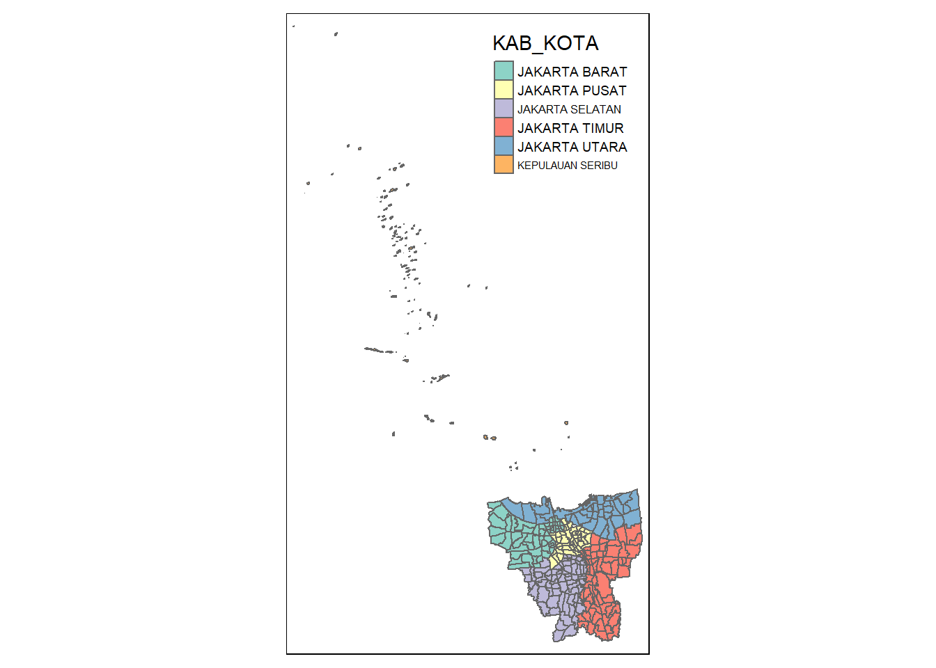
There are a few outer islands in Indonesia, and the ones closest according to Google are:
Kepulauan Seribu Utara (North Thousand Islands)
Kepulauan Seribu Selatan (South Thousand Islands)
We will see if there are any data in the KAB_KOTA (City Regency) that matches both.
unique(jakarta_village$"KAB_KOTA")[1] "JAKARTA BARAT" "JAKARTA PUSAT" "KEPULAUAN SERIBU" "JAKARTA UTARA"
[5] "JAKARTA TIMUR" "JAKARTA SELATAN" From the above, we can tell that Kepulauan Seribu (Thousand Islands) would encompass both Utara and Selatan (North and South)
We will exclude them from our dataset
jakarta_village <- filter(jakarta_village, KAB_KOTA != "KEPULAUAN SERIBU")Now we visualize to ensure there are no more outer islands
tmap_mode("plot")
tm_shape(jakarta_village) +
  tm_polygons("KAB_KOTA")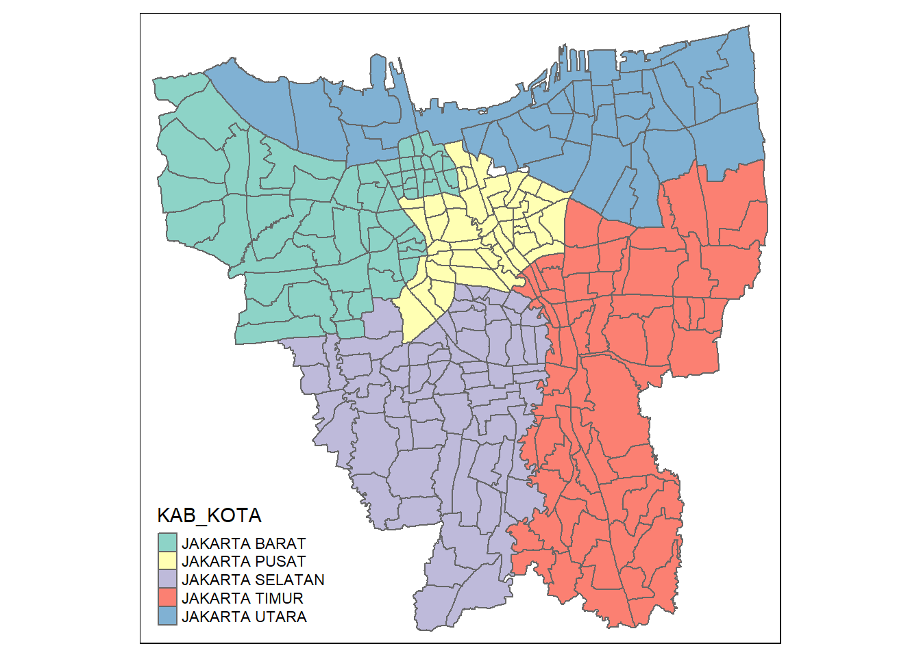
It appears they are removed!
Data-Preprocessing (Aspatial)
We need to process the dataset and only get the data we require. In this case, we need all the city/sub-district/ward areas. To data is cumulative, so we need to subtract from the previous month to get the current vaccinated. When downloaded, it appears that 28 Feb 2022 is missing. So, we’ll work with 27 for that month.
To get the number of vaccinated people, we take TARGET - NOT YET VACCINATED column.
We’ll take a look at the data we’re dealing with by importing the earliest one on July 2021
july2021 <- read_xlsx("data/vaccination/Data Vaksinasi Berbasis Kelurahan (31 Juli 2021).xlsx")We glimpse at the data:
glimpse(july2021)Rows: 268
Columns: 27
$ `KODE KELURAHAN` <chr> NA, "3172051003", "317304…
$ `WILAYAH KOTA` <chr> NA, "JAKARTA UTARA", "JAK…
$ KECAMATAN <chr> NA, "PADEMANGAN", "TAMBOR…
$ KELURAHAN <chr> "TOTAL", "ANCOL", "ANGKE"…
$ SASARAN <dbl> 8941211, 23947, 29381, 29…
$ `BELUM VAKSIN` <dbl> 4441501, 12333, 13875, 18…
$ `JUMLAH\r\nDOSIS 1` <dbl> 4499710, 11614, 15506, 10…
$ `JUMLAH\r\nDOSIS 2` <dbl> 1663218, 4181, 4798, 3658…
$ `TOTAL VAKSIN\r\nDIBERIKAN` <dbl> 6162928, 15795, 20304, 14…
$ `LANSIA\r\nDOSIS 1` <dbl> 502579, 1230, 2012, 865, …
$ `LANSIA\r\nDOSIS 2` <dbl> 440910, 1069, 1729, 701, …
$ `LANSIA TOTAL \r\nVAKSIN DIBERIKAN` <dbl> 943489, 2299, 3741, 1566,…
$ `PELAYAN PUBLIK\r\nDOSIS 1` <dbl> 1052883, 3333, 2586, 2837…
$ `PELAYAN PUBLIK\r\nDOSIS 2` <dbl> 666009, 2158, 1374, 1761,…
$ `PELAYAN PUBLIK TOTAL\r\nVAKSIN DIBERIKAN` <dbl> 1718892, 5491, 3960, 4598…
$ `GOTONG ROYONG\r\nDOSIS 1` <dbl> 56660, 78, 122, 174, 71, …
$ `GOTONG ROYONG\r\nDOSIS 2` <dbl> 38496, 51, 84, 106, 57, 7…
$ `GOTONG ROYONG TOTAL\r\nVAKSIN DIBERIKAN` <dbl> 95156, 129, 206, 280, 128…
$ `TENAGA KESEHATAN\r\nDOSIS 1` <dbl> 76397, 101, 90, 215, 73, …
$ `TENAGA KESEHATAN\r\nDOSIS 2` <dbl> 67484, 91, 82, 192, 67, 3…
$ `TENAGA KESEHATAN TOTAL\r\nVAKSIN DIBERIKAN` <dbl> 143881, 192, 172, 407, 14…
$ `TAHAPAN 3\r\nDOSIS 1` <dbl> 2279398, 5506, 9012, 5408…
$ `TAHAPAN 3\r\nDOSIS 2` <dbl> 446028, 789, 1519, 897, 4…
$ `TAHAPAN 3 TOTAL\r\nVAKSIN DIBERIKAN` <dbl> 2725426, 6295, 10531, 630…
$ `REMAJA\r\nDOSIS 1` <dbl> 531793, 1366, 1684, 1261,…
$ `REMAJA\r\nDOSIS 2` <dbl> 4291, 23, 10, 1, 1, 8, 6,…
$ `REMAJA TOTAL\r\nVAKSIN DIBERIKAN` <dbl> 536084, 1389, 1694, 1262,…We only require the first 6 column, and we need to create two more columns. We also remove the first row as that is not necessary
- Number vaccinated cumulatively
- Month
Once we have the number vaccinated cumulatively for that month, we can drop both ‘SASARAN’ and ‘BELUM VAKSIN’.
july2021 <- dplyr::select(july2021, 1:6) %>%
  dplyr::slice(-1) %>%
  mutate(total_vaccinated = `SASARAN` - `BELUM VAKSIN`) %>%
  mutate(month = dmy("31-Jul-2021")) %>%
  dplyr::select(-SASARAN, -`BELUM VAKSIN`)
Check if our data is correct:
july2021# A tibble: 267 × 6
`KODE KELURAHAN` `WILAYAH KOTA` KECAMATAN KELURA…¹ total…² month
<chr> <chr> <chr> <chr> <dbl> <date>
1 3172051003 JAKARTA UTARA PADEMANGAN ANCOL 11614 2021-07-31
2 3173041007 JAKARTA BARAT TAMBORA ANGKE 15506 2021-07-31
3 3175041005 JAKARTA TIMUR KRAMAT JATI BALE KA… 10760 2021-07-31
4 3175031003 JAKARTA TIMUR JATINEGARA BALI ME… 4579 2021-07-31
5 3175101006 JAKARTA TIMUR CIPAYUNG BAMBU A… 12510 2021-07-31
6 3174031002 JAKARTA SELATAN MAMPANG PRAPATAN BANGKA 11123 2021-07-31
7 3175051002 JAKARTA TIMUR PASAR REBO BARU 13823 2021-07-31
8 3175041004 JAKARTA TIMUR KRAMAT JATI BATU AM… 19050 2021-07-31
9 3171071002 JAKARTA PUSAT TANAH ABANG BENDUNG… 11516 2021-07-31
10 3175031002 JAKARTA TIMUR JATINEGARA BIDARA … 14905 2021-07-31
# … with 257 more rows, and abbreviated variable names ¹KELURAHAN,
# ²total_vaccinatedNow we will create a function to handle the pre-processing of the data. Mainly translating from Indonesian to English and apply the date into the tibble dataframe.
Pre-processing Function
The following function will apply the months and date, and also apply the rates of change as defined:
(TARGET - NOT VAX) / TARGET * 100
file_list <- list.files(path = "data/vaccination", pattern = "*.xlsx", full.names=TRUE)

process_aspatial_file <- function(file_name) {

    #Get the month and year of the file
    pattern <- "(\\b\\d{1,2}\\D{0,3})?\\b(?:Jan(?:uari)?|Feb(?:ruari)?|Mar(?:et)?|Apr(?:il)?|Mei|Jun(?:i)?|Jul(?:i)?|Agu(?:stus)?|Sep(?:tember)?|Okt(?:ober)?|(Nov|Des)(?:ember)?)\\D?(\\d{1,2}\\D?)?\\D?((19[7-9]\\d|20\\d{2})|\\d{2})"


    month_dict <- c("Januari"="January","Februari"="February","Maret"="March",
                "April"="April", "Mei"="May", "Juni"="June","Juli"="July",
                "Agustus"="August", "September"="September", "Oktober"="October"                  ,"November"="November","Desember"="December")

    matches <- str_extract(file_name, regex(pattern))
    replaced_eng <- str_replace_all(matches, month_dict)
    month_year <- dmy(replaced_eng)
    #month_year_string <- format(month_year, "%d-%m-%Y")

    #Calculate the vaccination
    vax_data <- read_xlsx(file_name)
    vax_data <- dplyr::select(vax_data, 1:6) %>%
                dplyr::slice(-1) %>%
                mutate(total_vaccinated_rate = (((`SASARAN` - `BELUM VAKSIN`) / `SASARAN`))*100) %>%
                mutate(month = month_year) %>%
                dplyr::select(-SASARAN, -`BELUM VAKSIN`)

    return(vax_data)

  }
dflist <- lapply(seq_along(file_list), function(x) process_aspatial_file(file_list[x]))Get the datatable for the entire Jakarta
vacc_jakarta <- ldply(dflist, data.frame)Rename the Indonesia names and sort the month column for better understanding:
vacc_jakarta <- vacc_jakarta %>%
  dplyr::rename(
    `village_code`=`KODE.KELURAHAN`,
    `city_area`=`WILAYAH.KOTA`,
    `sub_district`=KECAMATAN,
    `village`=KELURAHAN
    ) %>%
  arrange(month)
Check if there are any NA values
vacc_jakarta[rowSums(is.na(vacc_jakarta))!=0,][1] village_code city_area sub_district
[4] village total_vaccinated_rate month
<0 rows> (or 0-length row.names)None! We’ll pivot the rows of the dates into columns so it resembles a timeline
Note that it is a cumulative curve, where the vaccination rates will increase every month.
vacc_jakarta <- vacc_jakarta %>%
                    pivot_wider(names_from=month,
                                values_from=total_vaccinated_rate)
We’re done with the Aspatial side, now to combine both the geospatial and aspatial data
Combining Geospatial and Aspatial Data:
From the two datasets, it appears that a good place to perform inner join of the two tables would the the village level. (DESA_KELUR & village)
But first, we need to check to see if they are any discrepancies first before we perform the inner join.
jakarta_village_subdis <- c(jakarta_village$DESA_KELUR)
vacc_jakarta_subdis <- c(vacc_jakarta$village)

#Check if they are not in each other
unique(jakarta_village_subdis[!(jakarta_village_subdis %in% vacc_jakarta_subdis)])
[1] "KRENDANG" "RAWAJATI" "TENGAH"
[4] "BALEKAMBANG" "PINANGRANTI" "JATIPULO"
[7] "PALMERIAM" "KRAMATJATI" "HALIM PERDANA KUSUMA"#Check if they are not in each other
unique(vacc_jakarta_subdis[!(vacc_jakarta_subdis %in% jakarta_village_subdis)]) [1] "BALE KAMBANG" "HALIM PERDANA KUSUMAH" "JATI PULO"
[4] "KAMPUNG TENGAH" "KERENDANG" "KRAMAT JATI"
[7] "PAL MERIAM" "PINANG RANTI" "PULAU HARAPAN"
[10] "PULAU KELAPA" "PULAU PANGGANG" "PULAU PARI"
[13] "PULAU TIDUNG" "PULAU UNTUNG JAWA" "RAWA JATI" There appears to be a mismatch. There are some villages that are NOT present in the vaccine data
MISSING VILLAGES IN VACCINE DATA:
| Missing Villages |
|---|
| PULAU KELAPA |
| PULAU HARAPAN |
| PULAU PARI |
| PULAU TIDUNG |
| PULAU UNTUNG JAWA |
| PULAU PANGGANG |
These are villages from the outer islands, therefore should be excluded, but inner join operation will automatically drop and exclude them. So we do not need to worry about them!
We need to change and modify the following: (From quick research, it appears there are some spelling errors on the aspatial data side)
| Geospatial | Aspatial |
|---|---|
| BALEKAMBANG | BALE KAMBANG |
| HALIM PERDANA KUSUMA | HALIM PERDANA KUSUMAH (Error) |
| JATIPULO | JATI PULO |
| KRENDANG | KERENDANG (Error) |
| KRAMATJATI | KRAMAT JATI |
| PALMERIAM | PAL MERIAM |
| PINANGRANTI | PINANG RANTI |
| TENGAH | KAMPUNG TENGAH |
| RAWAJATI | RAWA JATI |
Make the modifications:
We will change the vacc_jakarta set as there are misspellings (Kerendang should be Krendang) in the vacc_jakarta set to match with the geospatial set.
vacc_jakarta$village[vacc_jakarta$village == 'BALE KAMBANG'] <- 'BALEKAMBANG'
vacc_jakarta$village[vacc_jakarta$village == 'HALIM PERDANA KUSUMAH'] <- 'HALIM PERDANA KUSUMA'
vacc_jakarta$village[vacc_jakarta$village == 'JATI PULO'] <- 'JATIPULO'
vacc_jakarta$village[vacc_jakarta$village == 'KERENDANG'] <- 'KRENDANG'
vacc_jakarta$village[vacc_jakarta$village == 'KRAMAT JATI'] <- 'KRAMATJATI'
vacc_jakarta$village[vacc_jakarta$village == 'PAL MERIAM'] <- 'PALMERIAM'
vacc_jakarta$village[vacc_jakarta$village == 'PINANG RANTI'] <- 'PINANGRANTI'
vacc_jakarta$village[vacc_jakarta$village == 'KAMPUNG TENGAH'] <- 'TENGAH'
vacc_jakarta$village[vacc_jakarta$village == 'RAWA JATI'] <- 'RAWAJATI'
Check again to make sure modification are done correctly:
jakarta_village_subdis <- c(jakarta_village$DESA_KELUR)
vacc_jakarta_subdis <- c(vacc_jakarta$village)

unique(jakarta_village_subdis[!(jakarta_village_subdis %in% vacc_jakarta_subdis)])character(0)unique(vacc_jakarta_subdis[!(vacc_jakarta_subdis %in% jakarta_village_subdis)])[1] "PULAU HARAPAN" "PULAU KELAPA" "PULAU PANGGANG"
[4] "PULAU PARI" "PULAU TIDUNG" "PULAU UNTUNG JAWA"All good, now we can perform inner join.
combined_jakarta <- left_join(jakarta_village, vacc_jakarta,
                              by=c("DESA_KELUR"="village"))

combined_jakarta <- combined_jakarta %>%
  dplyr::select(1:9, 13:24)
Visualize the Monthly Rate of Vaccination:
trace_val <- c("2021-07-31", "2021-08-31", "2021-09-30", "2021-10-31", "2021-11-30", "2021-12-31", "2022-01-31", "2022-02-27", "2022-03-31", "2022-04-30", "2022-05-31", "2022-06-30")

plot_creation <- function(df, month_name){
  tmap_mode("plot")
  tm_shape(df) +
    tm_borders(alpha=0.5)+
    tm_fill(month_name,
            title="Vaccination Rate",
            breaks=c(37, 47, 57, 67, 75, 83, 90))+
  tm_layout(main.title = month_name,
          main.title.position = "center",
          main.title.size = 1.2,
          legend.height = 0.45,
          legend.width = 0.35,
          frame = TRUE)
}
View the map interactively (June 2022)
tmap_mode("view")+
tm_shape(combined_jakarta) +
    tm_borders(alpha=0.5)+
    tm_polygons("2022-06-30",
                id="DESA_KELUR",
                breaks=c(37, 47, 57, 67, 75, 83, 90),
title="Vaccination Rate")tmap_arrange(plot_creation(combined_jakarta, "2021-07-31"),
plot_creation(combined_jakarta, "2021-08-31"),
plot_creation(combined_jakarta, "2021-09-30"),
plot_creation(combined_jakarta, "2021-10-31"))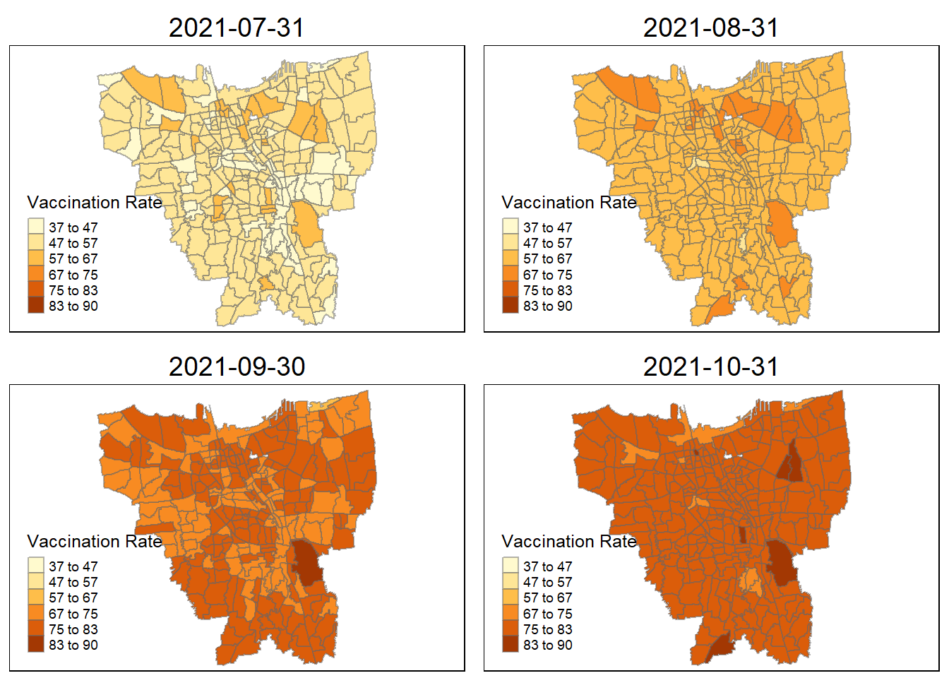
tmap_arrange(plot_creation(combined_jakarta, "2021-11-30"),
             plot_creation(combined_jakarta, "2021-12-31"),
             plot_creation(combined_jakarta, "2022-01-31"),
             plot_creation(combined_jakarta, "2022-02-27"))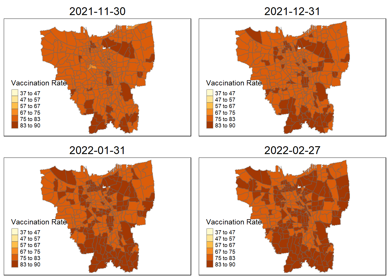
tmap_arrange(plot_creation(combined_jakarta, "2022-03-31"),
             plot_creation(combined_jakarta, "2022-04-30"),
             plot_creation(combined_jakarta, "2022-05-31"),
             plot_creation(combined_jakarta, "2022-06-30"))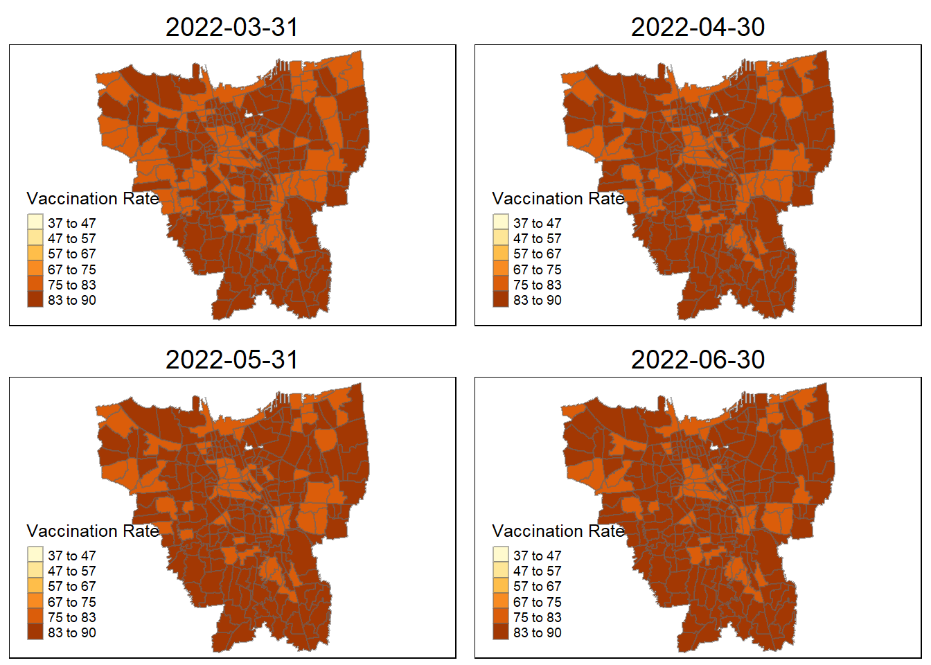
Describe the spatial patterns revealed by the maps:
From a glance, it appears that during the first three months, during 2021, only a few city states has a high rate of vaccination. However, in subsequent months, the neighboring village sub-district all begin to catch up save for a few. Eventually ending in 2022 June with most of the people vaccinated in Jakarta.
The village closest to the villages with higher vaccination rates are the second to start receiving the vaccination doses, as they show demonstrably higher vaccination rates compared to other villages (October 2021). They are then slowly doled out across nearby villages until most villages in Jakarta are almost fully vaccinated.
Interestingly, during this period of measure (July), there was an exponential spike (Reuters) in Covid-19 cases with heavy bans and movement restrictions across the board with recorded 2.2 million cases. This might explain why the almost equal distribution in terms of vaccination rates across the board in Jakarta. The only two villages, seemingly with lower rates compared to the rest of the city are:
Senayan
Kebon Melati
Petamburan
Local Gi* Analysis
Over here we will compute the local Gi* values for the monthly vaccination rates. Gi* only works for distance-based matrix and queen contiguity. This is to detect hot/cold spots for villages with high/low covid-19 vaccinations respectively. We will do it in a time-series to understand how the vaccinations are doled out across the country overtime.
Intepreting Gi* Values:
- Gi* > 0: Grouping of areas with values higher than average
- Gi* < 0: Grouping of areas with values lower than average
The values represents the intensity of grouping.
Set the seed for reproducebility
set.seed(1234)Create our Spatial-Temporal Cube
#Pivot long
jakarta_combined_long <- combined_jakarta %>%
  pivot_longer(cols=all_of(trace_val), names_to="Date", values_to = "total_vaccinated_rate") %>%
mutate(Date=as_date(Date))jakarta_combined_longSimple feature collection with 3132 features and 11 fields
Geometry type: MULTIPOLYGON
Dimension: XY
Bounding box: xmin: -3644275 ymin: 663887.8 xmax: -3606237 ymax: 701380.1
Projected CRS: DGN95 / Indonesia TM-3 zone 54.1
# A tibble: 3,132 × 12
OBJECT_ID KODE_DESA DESA KODE PROVI…¹ KAB_K…² KECAM…³ DESA_…⁴ JUMLA…⁵
* <dbl> <chr> <chr> <dbl> <chr> <chr> <chr> <chr> <dbl>
1 25477 3173031006 KEAGUNGAN 317303 DKI JA… JAKART… TAMAN … KEAGUN… 21609
2 25477 3173031006 KEAGUNGAN 317303 DKI JA… JAKART… TAMAN … KEAGUN… 21609
3 25477 3173031006 KEAGUNGAN 317303 DKI JA… JAKART… TAMAN … KEAGUN… 21609
4 25477 3173031006 KEAGUNGAN 317303 DKI JA… JAKART… TAMAN … KEAGUN… 21609
5 25477 3173031006 KEAGUNGAN 317303 DKI JA… JAKART… TAMAN … KEAGUN… 21609
6 25477 3173031006 KEAGUNGAN 317303 DKI JA… JAKART… TAMAN … KEAGUN… 21609
7 25477 3173031006 KEAGUNGAN 317303 DKI JA… JAKART… TAMAN … KEAGUN… 21609
8 25477 3173031006 KEAGUNGAN 317303 DKI JA… JAKART… TAMAN … KEAGUN… 21609
9 25477 3173031006 KEAGUNGAN 317303 DKI JA… JAKART… TAMAN … KEAGUN… 21609
10 25477 3173031006 KEAGUNGAN 317303 DKI JA… JAKART… TAMAN … KEAGUN… 21609
# … with 3,122 more rows, 3 more variables: geometry <MULTIPOLYGON [m]>,
# Date <date>, total_vaccinated_rate <dbl>, and abbreviated variable names
# ¹PROVINSI, ²KAB_KOTA, ³KECAMATAN, ⁴DESA_KELUR, ⁵JUMLAH_PENjakarta_combined_ts <- spacetime(jakarta_combined_long, jakarta_village,
.loc_col = "DESA_KELUR",
.time_col = "Date")Check if it’s a time cube
is_spacetime_cube(jakarta_combined_ts)[1] TRUESetting Contiguity Weight Matrices using Queen Method
For Local G* we will have to choose a distance weight matrix, whether it be fixed or inverse. In this case, we’re trying to map out how vaccines are doled out from respectively from villages with high vaccination rates. Therefore, we will use Inverse Distance
jakarta_combined_nb <- jakarta_combined_ts %>%
  activate("geometry") %>%
  mutate(nb = include_self(st_contiguity(geometry)),
         wt = st_inverse_distance(nb, geometry,
                                   scale=1,
                                   alpha=1),
         .before=1)%>%
  set_nbs("nb") %>%
set_wts("wt")jakarta_combined_nbSimple feature collection with 3132 features and 13 fields
Geometry type: MULTIPOLYGON
Dimension: XY
Bounding box: xmin: -3644275 ymin: 663887.8 xmax: -3606237 ymax: 701380.1
Projected CRS: DGN95 / Indonesia TM-3 zone 54.1
# A tibble: 3,132 × 14
OBJECT_ID KODE_DESA DESA KODE PROVI…¹ KAB_K…² KECAM…³ DESA_…⁴ JUMLA…⁵
* <dbl> <chr> <chr> <dbl> <chr> <chr> <chr> <chr> <dbl>
1 25477 3173031006 KEAGUNGAN 317303 DKI JA… JAKART… TAMAN … KEAGUN… 21609
2 25478 3173031007 GLODOK 317303 DKI JA… JAKART… TAMAN … GLODOK 9069
3 25397 3171031003 HARAPAN … 317103 DKI JA… JAKART… KEMAYO… HARAPA… 29085
4 25400 3171031006 CEMPAKA … 317103 DKI JA… JAKART… KEMAYO… CEMPAK… 41913
5 25390 3171021001 PASAR BA… 317102 DKI JA… JAKART… SAWAH … PASAR … 15793
6 25391 3171021002 KARANG A… 317102 DKI JA… JAKART… SAWAH … KARANG… 33383
7 25394 3171021005 MANGGA D… 317102 DKI JA… JAKART… SAWAH … MANGGA… 35906
8 25386 3171011003 PETOJO U… 317101 DKI JA… JAKART… GAMBIR PETOJO… 21828
9 25403 3171041001 SENEN 317104 DKI JA… JAKART… SENEN SENEN 8643
10 25408 3171041006 BUNGUR 317104 DKI JA… JAKART… SENEN BUNGUR 23001
# … with 3,122 more rows, 5 more variables: geometry <MULTIPOLYGON [m]>,
# Date <date>, total_vaccinated_rate <dbl>, nb <list>, wt <list>, and
# abbreviated variable names ¹PROVINSI, ²KAB_KOTA, ³KECAMATAN, ⁴DESA_KELUR,
# ⁵JUMLAH_PENVisualize the Queen Contiguity with Inverse Distance:
coords = st_coordinates(st_centroid(st_geometry(jakarta_combined_nb)))
plot(jakarta_combined_nb$nb, coords, pch = 19, cex = 0.6, col= "red")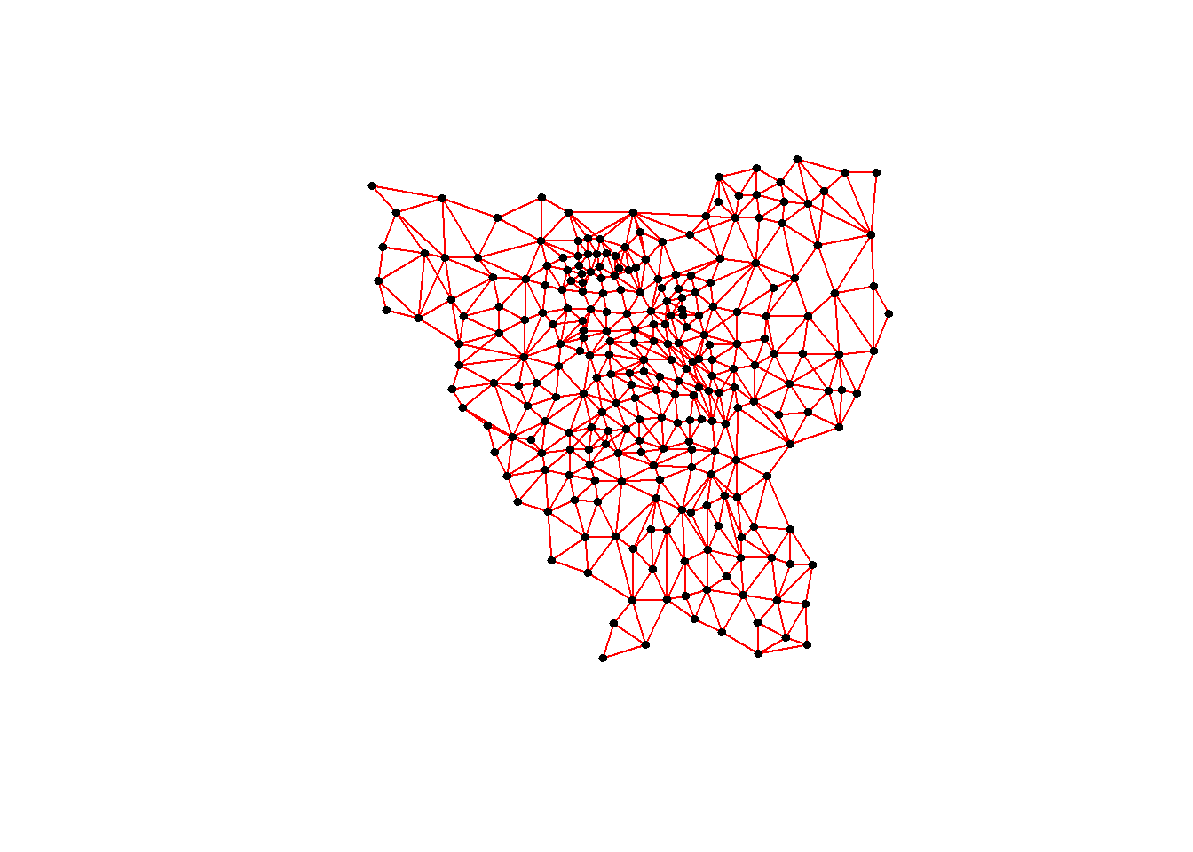
Calculate the G* for all the timeframe
Checking to ensure the output is correct
jakarta_HCSA <- jakarta_combined_nb %>%
  group_by(Date) %>%
  mutate(gi_star = local_gstar_perm(
    total_vaccinated_rate, nb, wt, nsim = 99)) %>%
tidyr::unnest(gi_star)jakarta_HCSASimple feature collection with 3132 features and 21 fields
Geometry type: MULTIPOLYGON
Dimension: XY
Bounding box: xmin: -3644275 ymin: 663887.8 xmax: -3606237 ymax: 701380.1
Projected CRS: DGN95 / Indonesia TM-3 zone 54.1
# A tibble: 3,132 × 22
# Groups: Date [12]
OBJECT_ID KODE_DESA DESA KODE PROVI…¹ KAB_K…² KECAM…³ DESA_…⁴ JUMLA…⁵
<dbl> <chr> <chr> <dbl> <chr> <chr> <chr> <chr> <dbl>
1 25477 3173031006 KEAGUNGAN 317303 DKI JA… JAKART… TAMAN … KEAGUN… 21609
2 25478 3173031007 GLODOK 317303 DKI JA… JAKART… TAMAN … GLODOK 9069
3 25397 3171031003 HARAPAN … 317103 DKI JA… JAKART… KEMAYO… HARAPA… 29085
4 25400 3171031006 CEMPAKA … 317103 DKI JA… JAKART… KEMAYO… CEMPAK… 41913
5 25390 3171021001 PASAR BA… 317102 DKI JA… JAKART… SAWAH … PASAR … 15793
6 25391 3171021002 KARANG A… 317102 DKI JA… JAKART… SAWAH … KARANG… 33383
7 25394 3171021005 MANGGA D… 317102 DKI JA… JAKART… SAWAH … MANGGA… 35906
8 25386 3171011003 PETOJO U… 317101 DKI JA… JAKART… GAMBIR PETOJO… 21828
9 25403 3171041001 SENEN 317104 DKI JA… JAKART… SENEN SENEN 8643
10 25408 3171041006 BUNGUR 317104 DKI JA… JAKART… SENEN BUNGUR 23001
# … with 3,122 more rows, 13 more variables: geometry <MULTIPOLYGON [m]>,
# Date <date>, total_vaccinated_rate <dbl>, nb <list>, wt <list>,
# gi_star <dbl>, e_gi <dbl>, var_gi <dbl>, p_value <dbl>, p_sim <dbl>,
# p_folded_sim <dbl>, skewness <dbl>, kurtosis <dbl>, and abbreviated
# variable names ¹PROVINSI, ²KAB_KOTA, ³KECAMATAN, ⁴DESA_KELUR, ⁵JUMLAH_PENMapping Gi* and show the Hot/Cold Spots
Now that we have the data, we can map our Gi* for analysis. This will show us how our hot and cold spot areas evolve over time. We will also exclude all statistically insignificant result.
jakarta_HCSA_sig <- jakarta_HCSA %>%
  filter(p_sim < 0.05)
create_gi_plot <- function(date_time) {
#Display the Gi* Vaccination Rate
tm_shape(filter(jakarta_HCSA, Date==date_time)) +
tm_polygons()+
tm_borders(alpha=0.5)+
tm_shape(filter(jakarta_HCSA_sig, Date==date_time)) +
tm_fill("gi_star")+
tm_borders(alpha=0.4)+
tm_layout(main.title = paste("Gi* Vax Rates", date_time))
}tmap_arrange(create_gi_plot("2021-07-31"),create_gi_plot("2021-08-31"))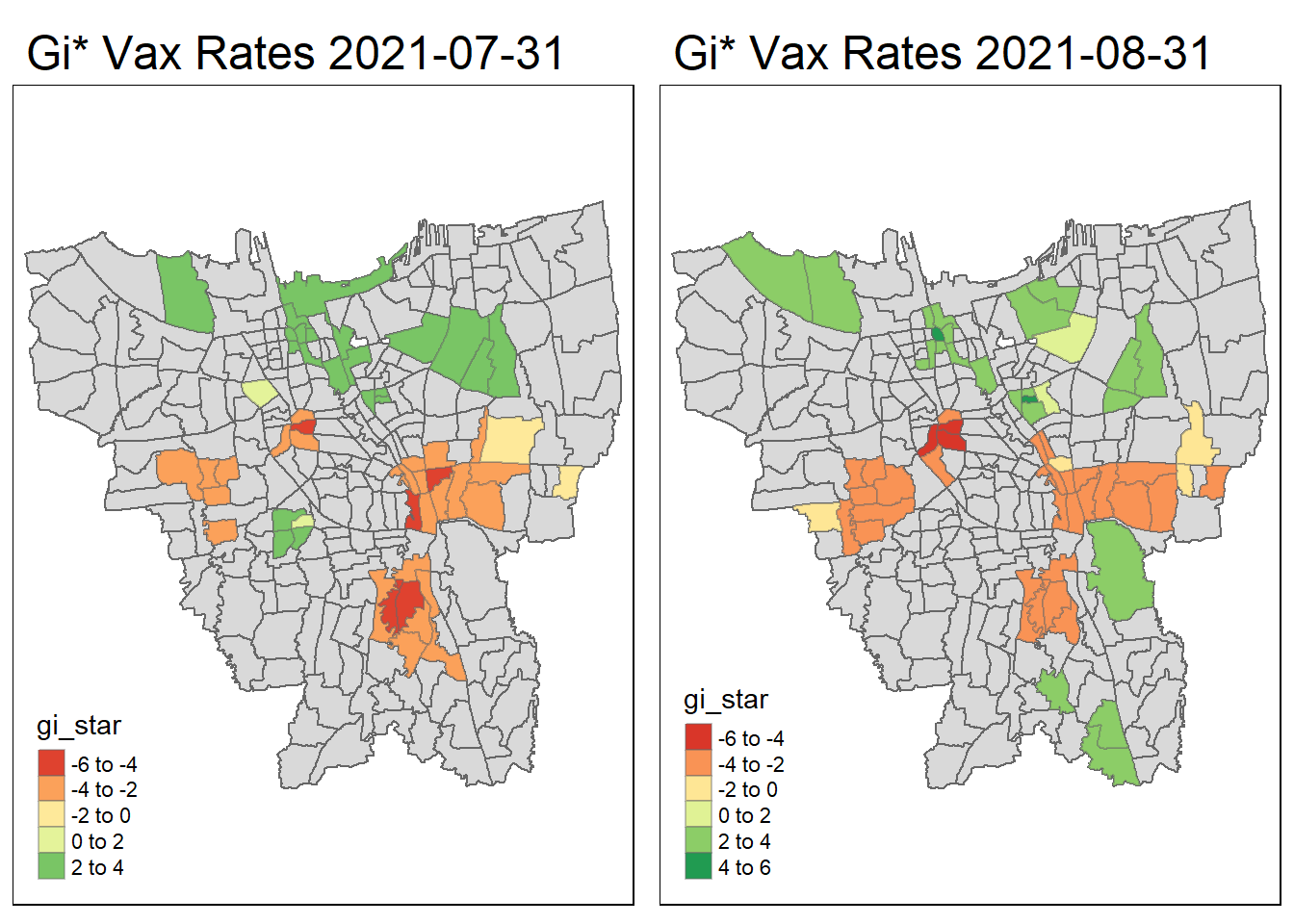
tmap_arrange(create_gi_plot("2021-09-30"),create_gi_plot("2021-10-31"))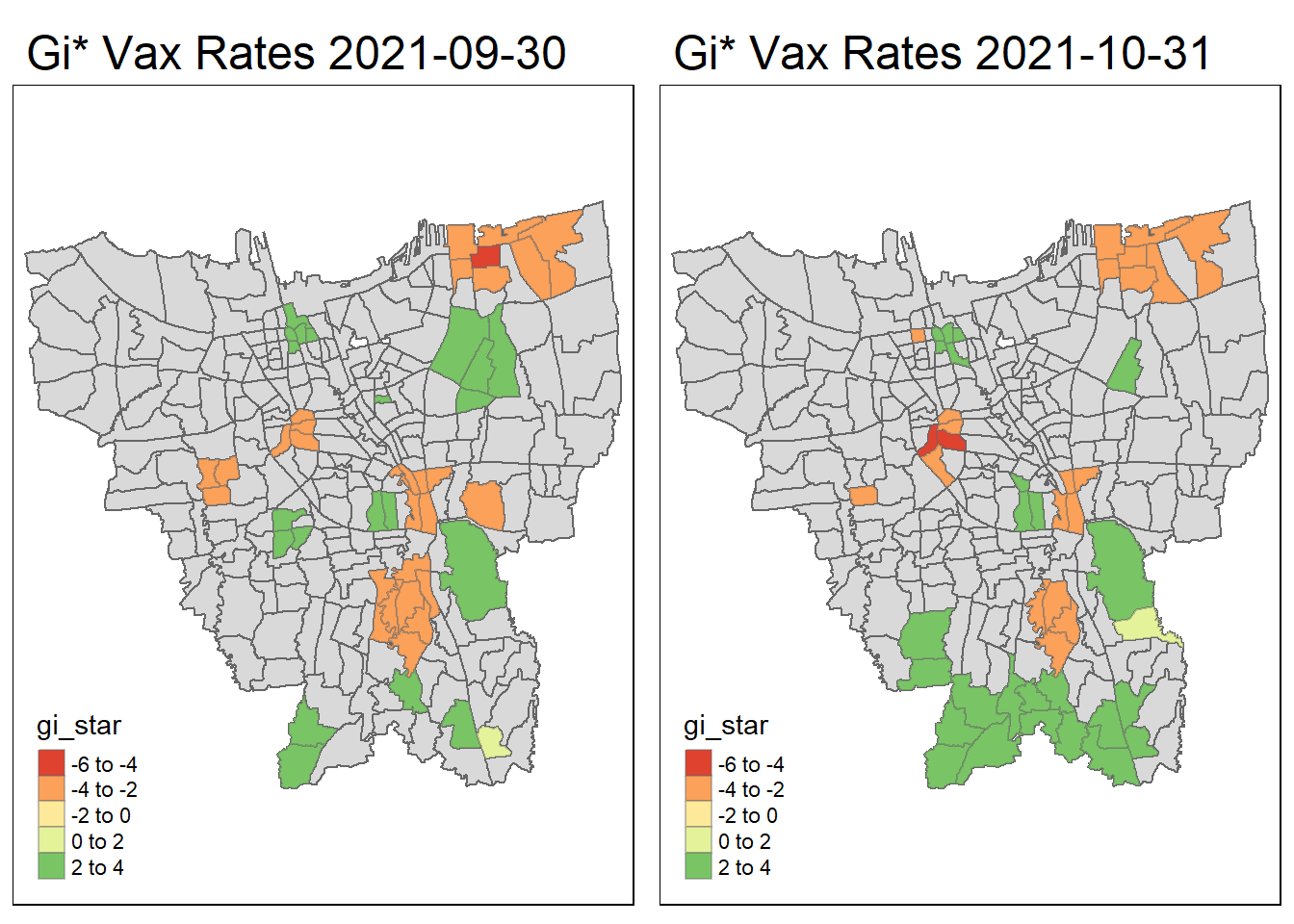
tmap_arrange(create_gi_plot("2021-11-30"),create_gi_plot("2021-12-31"))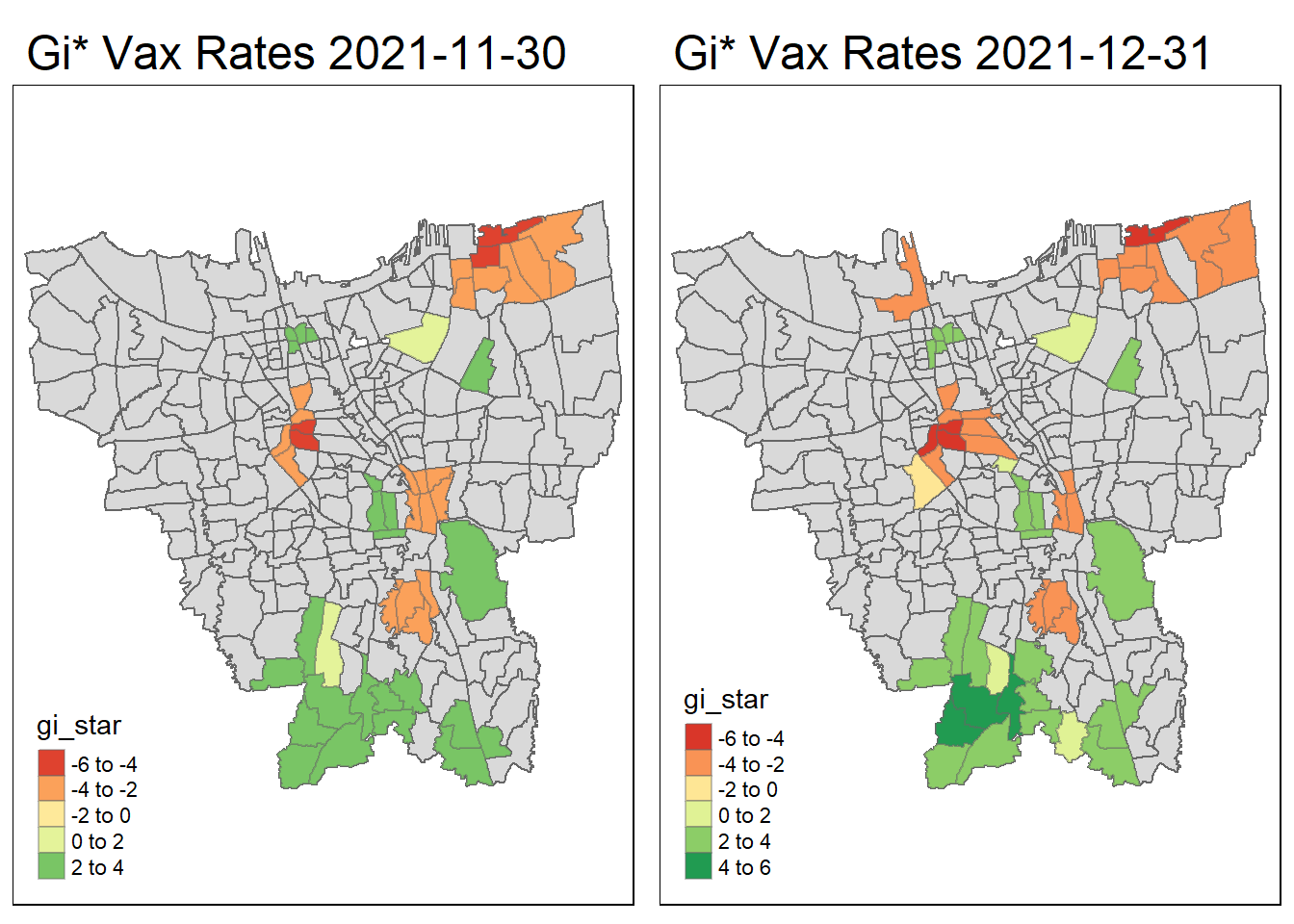
tmap_arrange(create_gi_plot("2022-01-31"),create_gi_plot("2022-02-27"))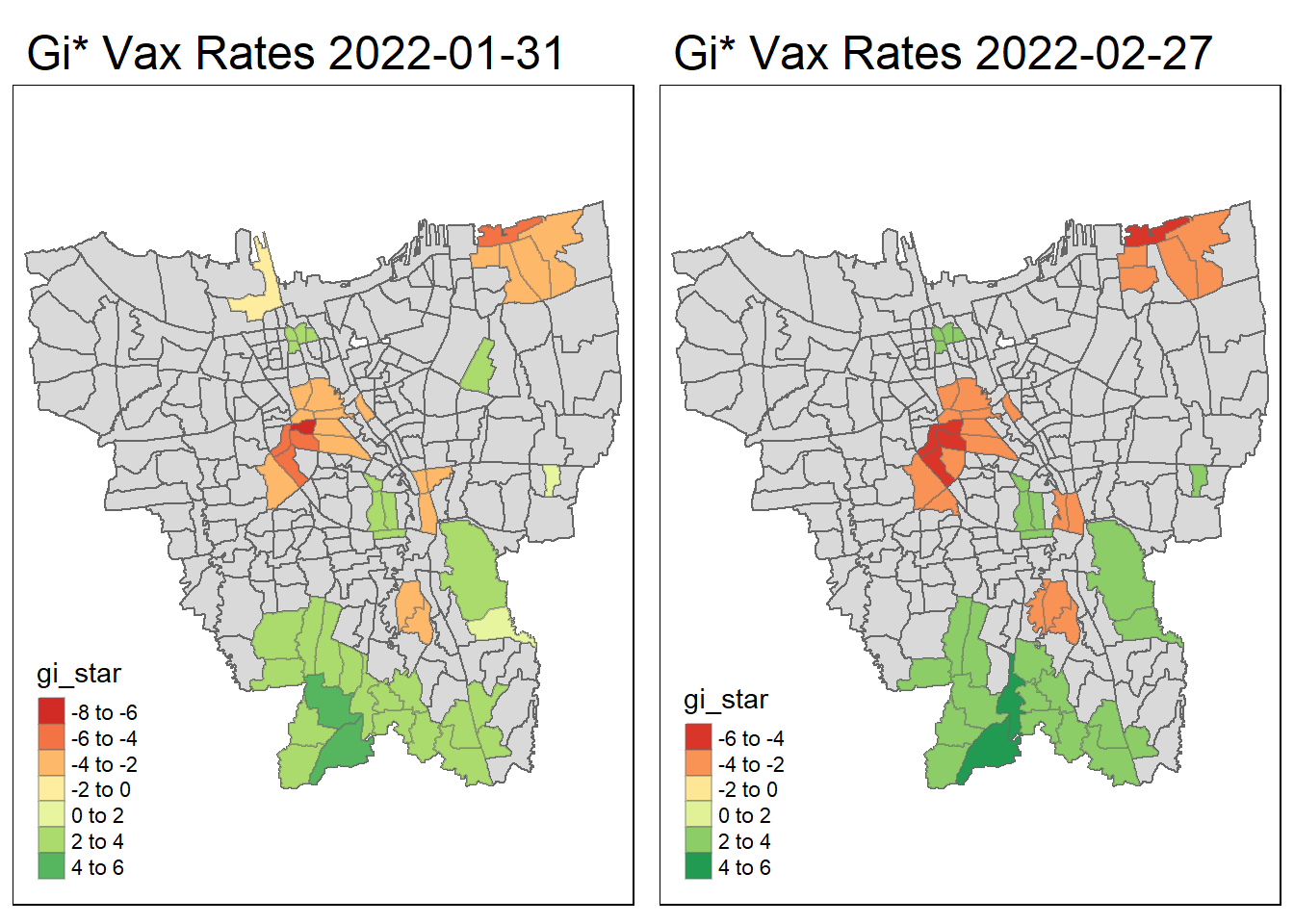
tmap_arrange(create_gi_plot("2022-03-31"),create_gi_plot("2022-04-30"))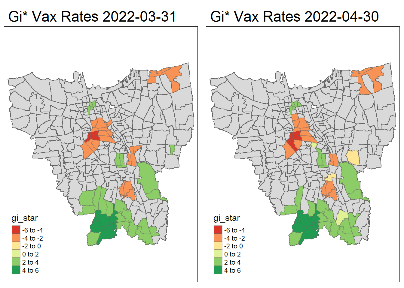
tmap_arrange(create_gi_plot("2022-05-31"),create_gi_plot("2022-06-30"))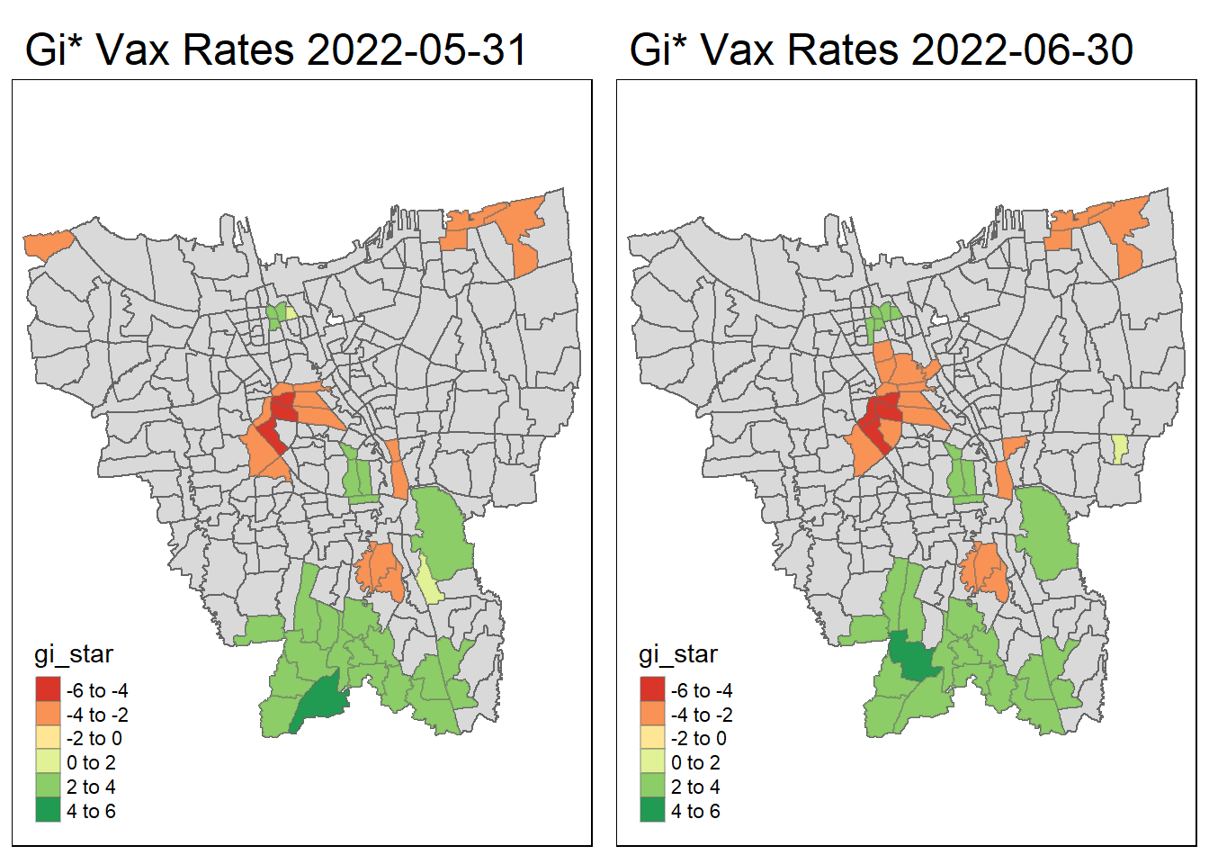
Interpreting the results
From the start, we can see that some villages from the North, Central, South, East and West Jakarta have high vaccination hot spot clusters, before moving to the southern part of Jakarta which encompasses a portion of East and South Jakarta.
Interestingly, Central Jakarta has the highest cluster of cold spots, where resistance towards the vaccine is high.
There could be a couple of reasons for the observed phenomena, first could be receptiveness. If we assume the vaccinations are doled out equally, we can suggest that the people in Central Jakarta are the least receptive compared to other areas. However, Central Jakarta and South Jakarta has the highest concentration of mid–high wealth individuals, which means its demographic should be relatively the same, but it produces such different results.
The more likely reason could be because these are disease hot spots, and they evolve over time, and the government is prioritizing areas where it is most ravaged by the virus. This explains the evolution of hot spots from north moving to south over time.
Man-Kendall Test
Based on the maps above, we will pick two hot spots and one cold spot for our analysis.
Hot Spot:
- Srengseng Sawah
- Lenteng Agung
Cold Spot:
- Kebon Kacang
Srengseng Sawah
srengseng <- jakarta_HCSA %>%
  ungroup() %>%
  filter(DESA_KELUR == "SRENGSENG SAWAH") %>%
  select(DESA_KELUR, Date, gi_star)
srengseng_p <- ggplot(data = srengseng,
aes(x = Date,
y = gi_star)) +
geom_line() +
theme_light()
ggplotly(srengseng_p)Lenteng Agung
lenteng <- jakarta_HCSA %>%
  ungroup() %>%
  filter(DESA_KELUR == "LENTENG AGUNG") %>%
  select(DESA_KELUR, Date, gi_star)
lenteng_p <- ggplot(data = lenteng,
aes(x = Date,
y = gi_star)) +
geom_line() +
theme_light()
ggplotly(lenteng_p)Srengseng Sawah and Lenteng Agung have similar upward positive trend. Given its statistical significance from our earlier analysis, we can say that the number of people receiving vaccination has a positive increase in trend over time that stabilized towards the end as most people get vaccinated.
This tells us that most people in these two villages are more receptive and willing towards receiving the vaccine (assuming vaccine availability is good) in its cluster.
Kebon Kacang
kebon <- jakarta_HCSA %>%
  ungroup() %>%
  filter(DESA_KELUR == "KEBON KACANG") %>%
  select(DESA_KELUR, Date, gi_star)
kebon_p <- ggplot(data = kebon,
aes(x = Date,
y = gi_star)) +
geom_line() +
theme_light()
ggplotly(kebon_p)From the result above, we can say there is a negative downward trend of people receiving the vaccination overtime. Therefore, we can say that the people in Kebon are not only initially resistant towards getting a vaccine, they are becoming increasingly resistant (again assuming vaccine availability is good), as the rate of people receiving vaccination continues on a downward spiral. There might be an underlying reason why this is the case. (Misinformation campaigns, lack of vaccine availability, lack of public health service announcements etc)
Together, we can suggest that there might be factors differentiating the villages the government might want to look into and identify the root cause for this difference.
Emerging Hotspot Analysis
Create a dataframe that only contains values we want to analyse
gi_star_jakarta <- jakarta_HCSA %>%
  select(8, 10,11:22)
ehsa <- gi_star_jakarta %>%
group_by(DESA_KELUR) %>%
summarise(mk=list(
unclass(
Kendall::MannKendall(gi_star)))) %>%
tidyr::unnest_wider(mk)Now we arrange to show the significant emerging hot/cold spots
emerging <- ehsa %>%
  arrange(sl, abs(tau)) %>%
  slice(1:5)
drp_jakarta_combined_ts <- jakarta_combined_ts %>% st_drop_geometry()ehsa <- emerging_hotspot_analysis(
x = drp_jakarta_combined_ts,
.var = "total_vaccinated_rate",
k = 1,
nsim = 99
)Visualize the distribution of the EHSA Classes
ggplot(data = ehsa,
       aes(x =classification, fill=classification)) +
  geom_bar()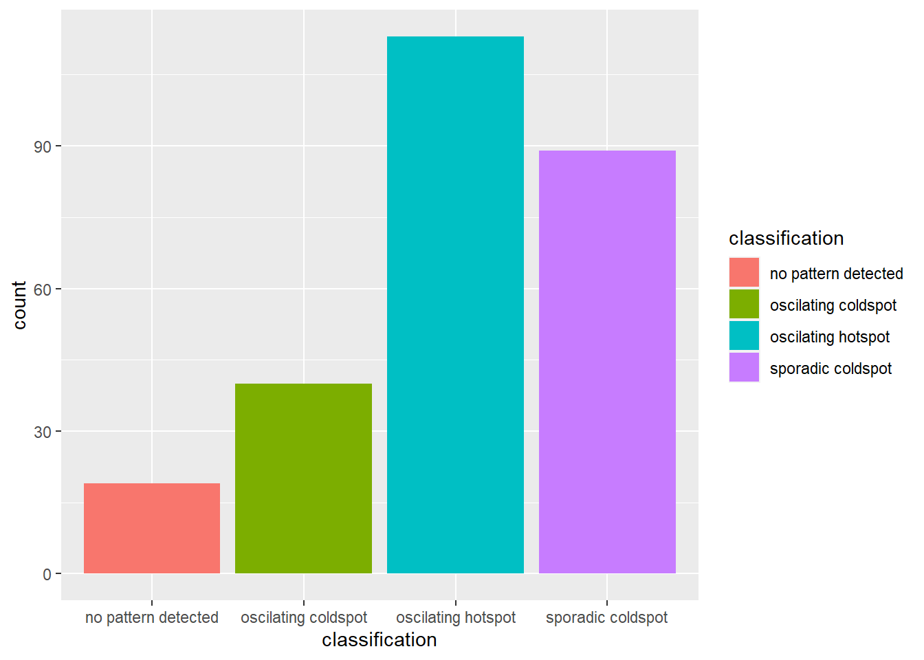
From the chart above, we can see that there are more villages with oscillating hot spots class compared to others.
Visualize EHSA in Jakarta
Now, we will visualize the geographic distribution of the EHSA classes. To do that, we will join together the jakarta_village shape file and the ehsa and also discard all insignificant results <0.05.
jakarta_ehsa <- jakarta_village %>%
  left_join(ehsa, by = c("DESA_KELUR" = "location"))
jakarta_ehsa_sig <- jakarta_ehsa %>%
filter(p_value < 0.05)
tmap_mode("plot")
tm_shape(jakarta_ehsa) +
tm_polygons() +
tm_borders(alpha = 0.5) +
tm_shape(jakarta_ehsa_sig) +
tm_fill("classification") +
tm_borders(alpha = 0.4)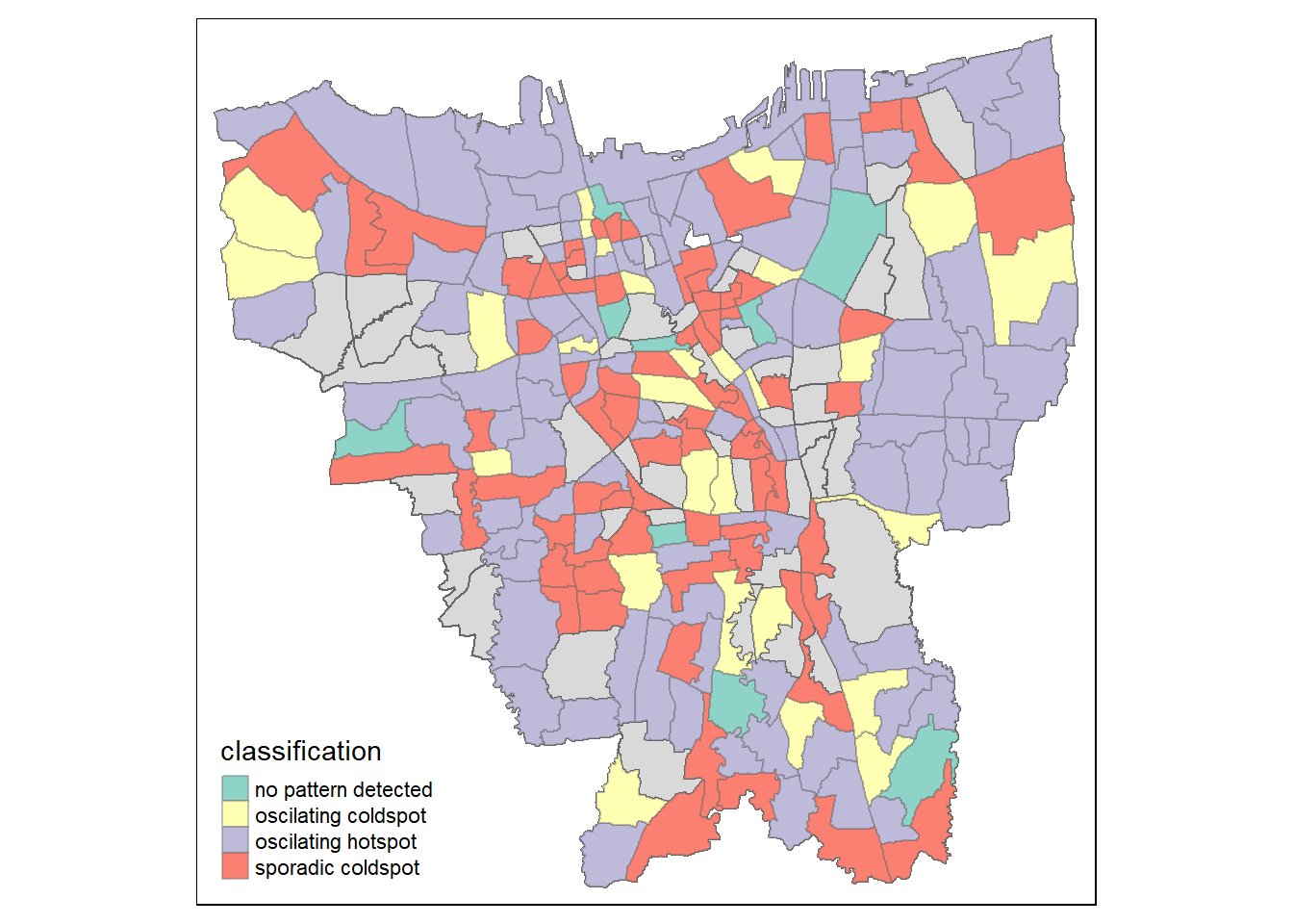
Describe the spatial patterns revealed:
From the graph above, it is immediately clear that the majority of the villages here have oscillating cold and hot spots. Oscillating in this context means there might be fluctuations of people getting vaccines and people not getting vaccines over time. This might suggest a vaccine availability problem or either that, a change in vaccine receptiveness/hesitancy, depending on hot or cold spot respectively in these areas.
A notable finding is that there is a sporadic cold spot in Srengseng Sawah, despite a positive trend in Gi* and the identification of a hot spot in the Man-Kendall test. How is this possible? This contradiction means that this cluster of districts have high vaccination rates in the surrounding area, but it itself is not part of a larger emerging hotspot with increasing vaccination rates as identified by the EHSA chart, as its surrounding are sporadic cold spots. It also indicates that the trend is NOT consistent, as we can tell from the Man-Kendall graph where the trend falls off towards the final time-step.
It might also reveal that vaccine availability is not consistent, even on a village level, despite Jakarta as a whole likely having higher availability compared to other states in Indonesia.
Overall, this highlights the importance of having to use multiple analysis in order to give a clearer picture into understanding the different spatial patterns and trends. It’s only with this that we can narrow down the factors contributing to vaccination rates in Jakarta.
Acknowledgement:
Prof Kam for all of his guidance and materials
Megan Sim, for code references on the data preparation of both the geospatial and aspatial data