pacman::p_load(maptools, sf, raster, spatstat, tmap)In-class Exercise 4
0.1 Loading the package
Things to learn from the code chunk
0.2 Importing Data
childcare_sf <- st_read("data/childcare.geojson") %>%
  st_transform(crs = 3414)
Reading layer `childcare' from data source
`D:\Documents\IS415-GAA-WY\inclass-ex\inclass-ex04\data\childcare.geojson'
using driver `GeoJSON'
Simple feature collection with 1545 features and 2 fields
Geometry type: POINT
Dimension: XYZ
Bounding box: xmin: 103.6824 ymin: 1.248403 xmax: 103.9897 ymax: 1.462134
z_range: zmin: 0 zmax: 0
Geodetic CRS: WGS 84sg_sf <- st_read(dsn = "data", layer="CostalOutline")Reading layer `CostalOutline' from data source
`D:\Documents\IS415-GAA-WY\inclass-ex\inclass-ex04\data' using driver `ESRI Shapefile'
Simple feature collection with 60 features and 4 fields
Geometry type: POLYGON
Dimension: XY
Bounding box: xmin: 2663.926 ymin: 16357.98 xmax: 56047.79 ymax: 50244.03
Projected CRS: SVY21mpsz_sf <- st_read(dsn = "data",
layer = "MP14_SUBZONE_WEB_PL")Reading layer `MP14_SUBZONE_WEB_PL' from data source
`D:\Documents\IS415-GAA-WY\inclass-ex\inclass-ex04\data' using driver `ESRI Shapefile'
Simple feature collection with 323 features and 15 fields
Geometry type: MULTIPOLYGON
Dimension: XY
Bounding box: xmin: 2667.538 ymin: 15748.72 xmax: 56396.44 ymax: 50256.33
Projected CRS: SVY21Notes:
Use tmap_mode(‘plot’) for staticmap
Change alpha of dots to change opacity for dots
Change view as vector
Also, there is an order to the way you display the tmap:
tmap_mode -> tmap_plot, shape, dots, view
tm_bubbles -> For proportion
tmap_mode('view') +
  tm_shape(childcare_sf)+
  tm_dots(alpha = 0.5)+
  tm_view(set.zoom.limits = c(11,14))
0.2.1 Convert from Shape File to Spatial Feature File
childcare <- as_Spatial(childcare_sf)
mpsz <- as_Spatial(mpsz_sf)
sg <- as_Spatial(sg_sf)
0.2.2 Convert from Spatial Feature to Generic
childcare_sp <- as(childcare, "SpatialPoints")
sg_sp <- as(sg, "SpatialPolygons")
0.2.3 Convert to PPP format (Spatstat)
Cos for points they need x y coordinates
childcare_ppp <- as(childcare_sp, "ppp")
childcare_ppp
Planar point pattern: 1545 points
window: rectangle = [11203.01, 45404.24] x [25667.6, 49300.88] unitsJitter to handle duplicate data
childcare_ppp_jit <- rjitter(childcare_ppp,
                             retry=TRUE,
                             nsim=1,
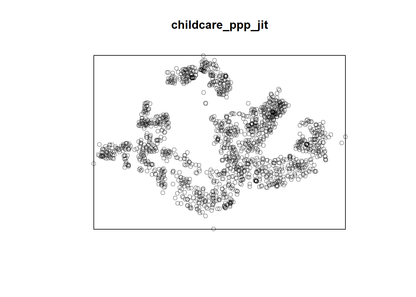
drop=TRUE)any(duplicated(childcare_ppp_jit))[1] FALSEplot(childcare_ppp_jit)
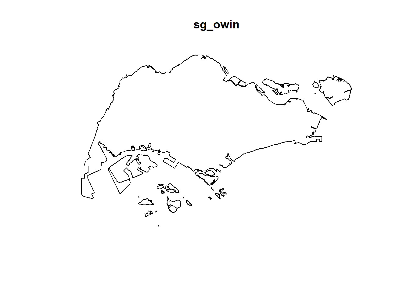
sg_owin <- as(sg_sp, "owin")
plot(sg_owin)
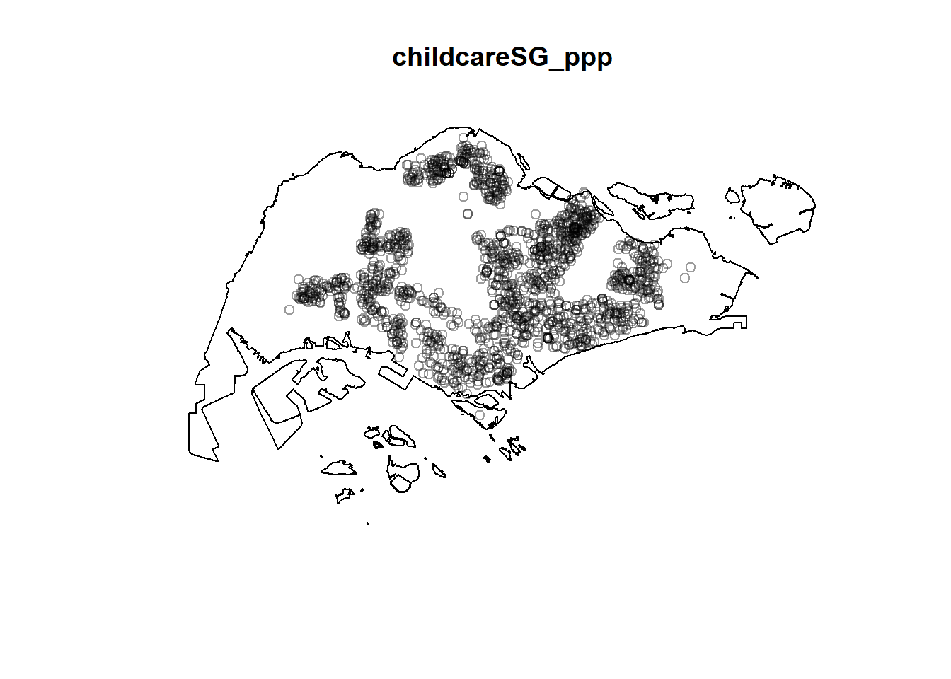
childcareSG_ppp = childcare_ppp[sg_owin]
plot(childcareSG_ppp)
Longer the bandwidth, the smoother it is.
If data points are well-distributed/well-defined, then fixed is better, adaptive otherwise
In the childcare sense, fixed is better because we know they typically cluster around residential areas
Use L function since that has a clearer interpretation (can maybe display all)
The number of monte carlo simulation we run will depend on our confidence level. (so if run 95 times, our confidence is 95% and 99 is 99%)
For L estimate:
The correction parameter is for H correction, but some might take longer to account for the edge. However, this alone cannot derive if the clustering is statistically significant
We run envelop which encompasses all the lines from the simulation
From exercise 5 (2nd order)
Anything within the envelop is statistically insignificant. Within the distance of 480-560 (outside the envelop), we see that is statistically significant and cluster. Below the 0 is no clustering.
All the lines are simulations of a 100 sample. (if we run 99 times).
The black line can be considered alpha-value that is compared to the p-value.
How to inteprete:
- At 480m distance between the childcare center, we can start to see signs of clustering.