pacman::p_load(sf, tidyverse, tmap, onemapsgapi, httr, jsonlite, olsrr, GWmodel, dotenv, matrixStats, spdep, SpatialML, Metrics, ggpubr)
#rsampleTake-Home Exercise 3
Background:
Singapore housing prices (HDB flats) are a form of public housing in Singapore that are designed to be affordable for the majority of the population. However, over the years, HDB prices have slowly been on the incline, influenced by various factors such as policies, locales, economic growth as well as its amenities and proximity to areas such as CBD. While there are policies in place by the government to stabilize pricing, they are still largely influenced by factors surrounding the HDB areas.
Packages used:
sf: Used for importing and processing geospatial data
tidyverse: A collection of packages to manipulate data
tmap: Used for creating thematic maps
onemapsapi: Used to query Singapore-specific spatial point data.
httr: Used for calling GET/POST requests for APIs
jsonlite: Used for parsing JSON files
olsrr: Used for building the Ordinary least squares model
GWmodel: Collection of spatial statistical methods - Mainly used for GWR and also its summary methods.
dotenv: Reading the API key from environment file
matrixStats: A convenient way to perform functions over rows and columns of matrices
spdep: Used to create spatial weights matrix objects.
SpatialML: A collection of packages. Mainly used to bandwidth calculations and performing geographically random forest methods.
Metrics: Used for calculating RMSE in our case.
corrplot: Used for mapping the Correlation plot, not included in pacman as there are some package issues
ggpubr: Used for data visualization and analysis
Loading in all the packages and data
Geospatial Data:
Singapore National Boundary and Master Plan 2019 subzone!
Singapore National Boundary is a polygon feature data showing the national boundary!
Master Plan 2019 subzone are information on URA 2019!
mpsz <- st_read(dsn="data/geospatial", "MPSZ-2019")
national_boundary <- st_read(dsn="data/geospatial", "CostalOutline")Aspatial Data
Resale Flat prices
Training dataset from 1st January 2021 to 31st December 2022
Test dataset from 1 January to the last day of February 2023 resale prices For our
For our case, we will be using four-room flats for our prediction
resale_flat <- read_csv("data/aspatial/resale-flat-prices-from-jan-2017-onwards.csv")Locational Factors:
For our assignment, we will need to look at location for
Proximity to CBD
Proximity to Eldercare
Proximity to Food court/Hawker
Proximity to MRT
Proximity to Park
Proximity to ‘Good’ primary schools
Proximity to Shopping Malls
Proximity to supermarket
Number of Kindergartens within 350m
Number of childcare centers within 350m
Number of primary schools within 1km
We start by sourcing some of this data
Geospatial Locational Source:
MRT/LRT and Bus Stop Locations
We can source from: LTA DataMall MRT/LRT Shapefile (It’s in Polygon!)
Bus Stop: LTA DataMall Bus Stop
mrt_lrt <- st_read(dsn="data/geospatial", layer="RapidTransitSystemStation")
bus_stop <- st_read(dsn="data/geospatial", layer="BusStop")There is something wrong, the MRT/LRT dataset is giving us polygon type rather than point. Despite the dataset saying it’s point.
OneMapSG Service API
We can extract the following according to their theme on OneMapSG API
Childcare (childcare)
Eldercare (eldercare)
Hawker Center (Queryname: hawkercentre)
Kindergarten (Queryname: Kindergartens)
Parks (Queryname: nationalparks)
Extra if we have time to think about:
Libraries (Queryname: libraries) [NUMBER WITHIN 350M]
Integrated Screening Programmes (queryname: moh_isp_clinics)
Tourist Attractions (Queryname: tourism) [NUMBER WITHIN 1KM]
Process of going through to create the shp file:
Courtesy of Megan’s work. (The following code chunk will be repeated to create the shp file for all the themes above).
#load_dot_env(file=".env")
#token <- Sys.getenv("TOKEN")
#themetibble <- get_theme(token, "themename")
#themetibble
#themesf <- st_as_sf(themetibble, coords=c("Lng", "Lat"), crs=4326)
#st_write(themesf, "themename.shp")Load in all the shp data
childcare <- st_read(dsn="data/geospatial", layer="childcare")
eldercare <- st_read(dsn="data/geospatial", layer="eldercare")
hawker_centre <- st_read(dsn="data/geospatial", layer="hawkercentre")
kindergarten <- st_read(dsn="data/geospatial", layer="kindergartens")
parks <- st_read(dsn="data/geospatial", layer="nationalparks")
libraries <- st_read(dsn="data/geospatial", layer="libraries")
isp_clinics <- st_read(dsn="data/geospatial", layer="moh_isp_clinics")
tourism <- st_read(dsn="data/geospatial", layer="tourism")External Sources
Supermarkets (Source: Dataportal)
Primary School (Wikipedia, Reverse Geocoded using OneMap API)
Top Primary Schools (We will pick the top 10 based off SchLah’s dataset)
Malls (Taken from this dataset) [NOTE: SVY21]
supermarkets <- st_read("data/geospatial/supermarkets.kml")Load Primary School Data with Lat/Long
The lat/long are taken from OneMapSG API
Top 10 schools as well, dervied from schlah
primary_sch <- read_csv("data/aspatial/primary_school_geo.csv")
top10_pri_sch <- read_csv("data/aspatial/top_10_primary_school_geo.csv")Load Shopping Malls
shopping_mall <- read_csv("data/aspatial/shopping_mall.csv")Data Wrangling (Geospatial)
List of task to do:
Convert some remaining data to Geospatial
Convert multipoint to point data (Removing the ‘z’) for supermarket
Convert all if not already in SVY21 into SVY21 (3414)
Remove all unnecessary columns
Check for null values
Convert all of our datasets from CSV to Geospatial (shp)
Primary Schools
Shopping Malls
Within primary school, the OneMapAPI is not able to properly return the correct coordinate as the name is ‘CATHOLIC HIGH SCHOOL (PRIMARY)’. For it to return the correct coordinate, the name has to be truncated without (PRIMARY).
primary_sch_sf <- st_as_sf(primary_sch, coords=c("LONG", "LAT"), crs=4326)
top_primary_sch_sf <- st_as_sf(top10_pri_sch, coords=c("LONG", "LAT"), crs=4326)shopping_mall_sf <- st_as_sf(shopping_mall, coords=c("longitude", "latitude"), crs=4326)Remove ‘Z-Dimension’ for Supermarket Data
supermarkets <- st_zm(supermarkets)Check and change all EPSG for Geospatial data to ESPG 3414
childcare3414 <- st_transform(childcare, crs=3414)
eldercare3414 <- st_transform(eldercare, crs=3414)
hawker_centre3414 <- st_transform(hawker_centre, crs=3414)
kindergarten3414 <- st_transform(kindergarten, crs=3414)
parks3414 <- st_transform(parks, crs=3414)
libraries3414 <- st_transform(libraries, crs=3414)
isp_clinics3414 <- st_transform(isp_clinics, crs=3414)
tourism3414 <- st_transform(tourism, crs=3414)
primary_sch_sf_3414 <- st_transform(primary_sch_sf, crs=3414)
top_primary_sch_sf_3414 <- st_transform(top_primary_sch_sf, crs=3414)
shopping_mall_sf_3414 <- st_transform(shopping_mall_sf, crs=3414)Check others:
st_crs(primary_sch_sf_3414)st_crs(top_primary_sch_sf_3414)st_crs(shopping_mall_sf_3414)st_crs(supermarkets)Looks like Supermarket is still in WGS84, let’s fix that
supermarkets3414 <- st_transform(supermarkets, crs=3414)Check to make sure…
st_crs(supermarkets3414)Remove all unnecessary columns
After glimpsing at the sf dataframe, we are going to remove all useless columns.
Information such as addresses/descriptions are not necessary, as all we need are the point data
We will keep the name for identification purposes
We will keep name and geometry
childcare3414 <- childcare3414 %>%
select(c('NAME', 'geometry'))Check result
childcare3414Same thing, name and geometry
eldercare3414 <- eldercare3414 %>%
select(c('NAME', 'geometry'))Check result
eldercare3414hawker_centre3414 <- hawker_centre3414 %>%
select(c('NAME', 'geometry'))hawker_centre3414isp_clinics3414 <- isp_clinics3414 %>%
select(c('NAME', 'geometry'))isp_clinics3414kindergarten3414 <- kindergarten3414 %>%
select(c('NAME', 'geometry'))kindergarten3414libraries3414 <- libraries3414 %>%
select(c('NAME', 'geometry'))libraries3414We only keep STN_NAM_DE and geometry
Note that the file is in polygon format, rather than point. Might have to deal with it.
https://stackoverflow.com/questions/52522872/r-sf-package-centroid-within-polygon
mrt_lrt <- mrt_lrt %>%
select(c('STN_NAM_DE', 'geometry'))Check
mrt_lrtparks3414 <- parks3414 %>%
select(c('NAME', 'geometry'))parks3414primary_sch_sf_3414 <- primary_sch_sf_3414 %>%
select(c('Primary school', 'geometry'))primary_sch_sfsupermarkets3414 <- supermarkets3414 %>%
select(c('Name', 'geometry'))supermarkets3414tourism3414 <- tourism3414 %>%
select(c('NAME', 'geometry'))tourism3414Dealing with the anomaly - MRT/LRT
Despite it saying that’s point data, it gives polygon data, therefore we need to convert the polygon into point data. Unfortunately, there appears to be an issue that causes st_make_valid to not work, due to missing data within the polygon (There is an ‘na’).
Thus, we’ll take this chance to do some fine tuning and make use of OneMapSG to return us the correct coordinates. We will also remove all ‘depots’ as they are not considered MRT/LRTs for our dataset.
mrt_lrt_new_set <- read_csv("data/aspatial/mrt_lrt_lat_long.csv")Convert into an SF Object
mrt_lrt_ns_sf <- st_as_sf(mrt_lrt_new_set, coords=c("LONG", "LAT"), crs=4326)mrt_lrt_ns_sf <- mrt_lrt_ns_sf %>%
select(c('STN_NAM_DE', 'geometry'))mrt_lrt_ns_sf_3414 <- st_transform(mrt_lrt_ns_sf, crs=3414)View the map to make sure the mapping is correct
tmap_mode("view")+
tm_shape(bus_stop)+
tm_dots(col="purple", size=0.05)Looks like we have some bus stations in Malaysia, which makes sense, as there are some Singapore buses that travel into Malaysia.
These stops are:
LARKIN TERMINAL (Malaysia) [46239]
KOTARAYA II TER [46609]
JB SENTRAL [47701]
JOHOR BAHRU CHECKPOINT (46211, 46219)
We don’t want them in our calculation, so we’ll remove them.
bus_stop_to_remove <- c(46239, 46609, 47701, 46211, 46219)
bus_stop_cleaned <- filter(bus_stop, !(BUS_STOP_N %in% bus_stop_to_remove))Check the map again:s
tm_shape(bus_stop_cleaned)+
tm_dots(col="purple", size=0.05)Convert Bus Stop from WGS84 to SVY21
bus_stop_cleaned_3414 <- st_transform(bus_stop_cleaned, crs = 3414)st_crs(bus_stop_cleaned_3414)Data Wrangling (Aspatial)
We will strictly be looking at Four Room Flats
Training Set: 1st January 2021 - 31st December 2022
Test Set: January - February 2023
resale_flat_sub <- filter(resale_flat,flat_type == "4 ROOM") %>%
filter(month >= "2021-01" & month <= "2023-02")Transforming the Data into usable data
Looking at the data, we will now need to combine both the block and street name to form the address so we can lookup for the postal code and retrieve the LAT/LONG
We will also need to calculate the remaining number of lease. Given that the remaining lease are in ‘YEAR’ + ‘MONTH’ format, we need to change it into a continuous number. We will change it to ‘MONTHS’.
rs_modified <- resale_flat_sub %>%
mutate(resale_flat_sub, address = paste(block,street_name)) %>%
mutate(resale_flat_sub, remaining_lease_yr = as.integer(str_sub(remaining_lease, 0, 2))) %>%
mutate(resale_flat_sub, remaining_lease_mth = as.integer(str_sub(remaining_lease, 9, 11)))Calculate the LEASE in Months and remove all intermediary columns
Convert all NA into 0
Sum up YEAR and MONTH and place them into a new column
Select only the columns we need.
rs_modified$remaining_lease_mth[is.na(rs_modified$remaining_lease_mth)] <- 0
rs_modified$remaining_lease_yr <- rs_modified$remaining_lease_yr * 12
rs_modified <- rs_modified %>%
mutate(remaining_lease_mths = rowSums(rs_modified[, c("remaining_lease_yr", "remaining_lease_mth")])) %>%
select(month, town, address, block, street_name, flat_type, storey_range, floor_area_sqm, flat_model,
lease_commence_date, remaining_lease_mths, resale_price)Glimpse at our data:
glimpse(rs_modified)Retrieving the LAT/LONG Coordinates from OneMap.sg API
The following solution is courtesy of: Nor Aisyah
We first create a unique list of addresses
add_list <- sort(unique(rs_modified$address))Now we will focus on getting the data needed.
In the following code chunk, the goal is to retrieve coordinates for a given search value using OneMap SG’s REST APIs. The code creates a dataframe to store the final retrieved coordinates and uses the httr package’s GET() function to make a GET request to https://developers.onemap.sg/commonapi/search.
The required variables to be included in the GET request are searchVal, returnGeom {Y/N}, and getAddrDetails {Y/N}.
The JSON response returned will contain multiple fields, but we are only interested in the postal code and coordinates like Latitude & Longitude. A new dataframe is created to store each final set of coordinates retrieved during the loop, and the number of responses returned is checked to append to the main dataframe accordingly. Invalid addresses are also checked, and the response is appended to the main dataframe using rbind() function of base R package.
retrieve_coords <- function(add_list){
# Create a data frame to store all retrieved coordinates
postal_coords <- data.frame()
for (i in add_list){
#print(i)
r <- GET('https://developers.onemap.sg/commonapi/search?',
query=list(searchVal=i,
returnGeom='Y',
getAddrDetails='Y'))
data <- fromJSON(rawToChar(r$content))
found <- data$found
res <- data$results
# Create a new data frame for each address
new_row <- data.frame()
# If single result, append
if (found == 1){
postal <- res$POSTAL
lat <- res$LATITUDE
lng <- res$LONGITUDE
new_row <- data.frame(address= i, postal = postal, latitude = lat, longitude = lng)
}
# If multiple results, drop NIL and append top 1
else if (found > 1){
# Remove those with NIL as postal
res_sub <- res[res$POSTAL != "NIL", ]
# Set as NA first if no Postal
if (nrow(res_sub) == 0) {
new_row <- data.frame(address= i, postal = NA, latitude = NA, longitude = NA)
}
else{
top1 <- head(res_sub, n = 1)
postal <- top1$POSTAL
lat <- top1$LATITUDE
lng <- top1$LONGITUDE
new_row <- data.frame(address= i, postal = postal, latitude = lat, longitude = lng)
}
}
else {
new_row <- data.frame(address= i, postal = NA, latitude = NA, longitude = NA)
}
# Add the row
postal_coords <- rbind(postal_coords, new_row)
}
return(postal_coords)
}We call the function to get the coordinates
coords <- retrieve_coords(add_list)Inspect the results
coords[(is.na(coords$postal) | is.na(coords$latitude) | is.na(coords$longitude) | coords$postal=="NIL"), ]From the results, we can see that it has missing postal code. However, the postal code is not as relevant to our analysis as latitude and longitude.
The missing respective postal code are:
680215
680216
rs_coords <- left_join(rs_modified, coords, by = c('address' = 'address'))Write file to RDS
write_rds(rs_coords, "data/aspatial/rs_coords.rds")Read the RDS file
resale_sub_flat <- read_rds("data/aspatial/rs_coords.rds")Assign and transform CRS
Data from OneMapSG are in WGS84, as evident from the decimal. So we will create a SF object in that code before transforming into SVY21
resale_coords_sf <- st_as_sf(resale_sub_flat,
coords = c("longitude",
"latitude"),
crs=4326) %>%
st_transform(crs = 3414)st_crs(resale_coords_sf)Check if there are any NA outside of what we confirmed earlier
rows_with_na <- which(is.na(resale_coords_sf), arr.ind=TRUE)if (nrow(rows_with_na) > 0) {
message("The following rows have NA values:")
print(rows_with_na)
} else {
message("The dataframe does not contain any rows with NA values.")
}Remove all unnecessary rows
We only need to keep the identifier, time, resale price, spatial point data, and the structural factors as listed below
Area of Unit
Floor Level
Remaining Lease
Age of Unit
Note that we have not handled the age of unit yet. We’ll handle that later.
trim_resale_flat <- resale_coords_sf %>%
select(1:3, 6:8, 11:12)Determining CBD
We need to consider the distance to CBD as well. We will take ‘Downtown Core’ as our reference point, which is located in the southwest of Singapore.
cbd_lat <- 1.287953
cbd_long <- 103.851784
cbd_sf <- data.frame(cbd_lat, cbd_long) %>%
st_as_sf(coords = c("cbd_long", "cbd_lat"), crs=4326) %>%
st_transform(crs=3414)Proximity Distance Calculation
For our next step, we will need to integrate all of our geospatial data by calculating the proximity to the amenities.
The following function calculates proximity
- rowMins from matrixStats package finds the shortest possible distance within the distance matrix.
proximity <- function(df1, df2, varname) {
dist_matrix <- st_distance(df1, df2) %>%
units::drop_units()
df1[,varname] <- rowMins(dist_matrix)
return(df1)
}Implement the Proximity Calculations:
trim_resale_flat <- proximity(trim_resale_flat, cbd_sf, "PROX_CBD") %>%
proximity(., eldercare3414, "PROX_ELDERCARE") %>%
proximity(., hawker_centre3414, "PROX_HAWKER") %>%
proximity(., isp_clinics3414, "PROX_ISP") %>%
proximity(., mrt_lrt_ns_sf_3414, "PROX_MRT") %>%
proximity(., parks3414, "PROX_PARKS") %>%
proximity(., top_primary_sch_sf_3414, "PROX_TOP_PRI") %>%
proximity(., shopping_mall_sf_3414, "PROX_SHOPPING") %>%
proximity(., supermarkets3414, "PROX_SUPERMARKETS")Facility Count within Radius
In addition to calculating the shortest distance between points, we’re also interested in finding out how many facilities are located within a specific radius. To accomplish this, we’ll use the st_distance() function to calculate the distance between the flats and the desired facilities. We’ll then use rowSums() to add up the observations and obtain the count of facilities within the desired radius. The resulting values will be added to the data frame as a new column.
num_radius <- function(df1, df2, varname, radius) {
dist_matrix <- st_distance(df1, df2) %>%
units::drop_units() %>%
as.data.frame()
df1[,varname] <- rowSums(dist_matrix <= radius)
return(df1)
}Implement the function:
trim_resale_flat <-
num_radius(trim_resale_flat, kindergarten3414, "NUM_KINDERGARTEN", 350) %>%
num_radius(., childcare3414, "NUM_CHILDCARE", 350) %>%
num_radius(., bus_stop_cleaned_3414, "NUM_BUS_STOPS", 350) %>%
num_radius(., primary_sch_sf_3414, "NUM_PRI_SCHS", 1000) %>%
num_radius(., tourism3414, "NUM_TOURIST_SITES", 1000)Save the Data as RDS
Before we do that, we should trim the name, as when converting to RDS the column names are shortened due to limitations
trim_resale_flat <- trim_resale_flat %>%
mutate() %>%
rename("AREA_SQM" = "floor_area_sqm",
"LEASE_MTHS" = "remaining_lease_mths",
"PRICE"= "resale_price",
"FLAT" = "flat_type",
"STOREY" = "storey_range")st_write(trim_resale_flat, "data/geospatial/resale_flat_final.shp")Reimport by reloading our dataset
resale_flat_sf <- st_read(dsn="data/geospatial", layer="resale_flat_final") We’re done with gathering and creating our data! Now we can move onto our exploratory data analysis and building our prediction models. Note that there are still some data that need to be modified. Such as ordinal data like Storeys and also the calculation of the flat’s age.
Calculate age of unit
To calculate the age of unit, we will take 2023 (current year) - lease_commence_date to find out the age of the flat. Then we’ll append it into our new sf object.
resale_flat_sub_age <- resale_flat_sub %>%
mutate("age_of_unit" = 2023 - lease_commence_date)resale_flat_sf <- resale_flat_sf %>%
mutate("age_of_unit" = resale_flat_sub_age$age_of_unit)Speaking of which, we’ll handle them now.
Storey Data:
It’s a categorical data that has meaning when ordered. Higher/lower levels could potentially have an impact on the price of the HDB Flat. Therefore, we should convert this column of data into numbers, one that the regression can learn from.
storeys <- sort(unique(resale_flat_sf$STOREY))
storey_order <- 1:length(storeys)
storey_range_order <- data.frame(storeys, storey_order)storey_range_orderFrom the above, we can see that the storey values have been sorted from 1 - 10
We will combine this data with the base resale SF. Unfortunately, we have to drop the geometric column first before we can perform the join. So we’ll do that, then we’ll combine both the columns
geom_temp_store <- st_geometry(resale_flat_sf)
temp_no_geo <- st_drop_geometry(resale_flat_sf)
temp_join <- dplyr::left_join(temp_no_geo, storey_range_order, by=c("STOREY"= "storeys"))
final_resale_output <- st_as_sf(temp_join, geom_temp_store)final_resale_outputWrite and read file
write_rds(final_resale_output, "data/model/final_resale_output.rds")final_resale_output <- read_rds("data/model/final_resale_output.rds")Rename to Columns so they are more readable
Due to abbreviation from Shapefile limitation, we will rename them back so it’s readable.
final_resale_output <- final_resale_output %>%
mutate() %>%
rename("PROX_CBD" = "PROX_CB",
"PROX_ELDERCARE" = "PROX_EL",
"PROX_HAWKER"= "PROX_HA",
"PROX_ISP" = "PROX_IS",
"PROX_MRT" = "PROX_MR",
"PROX_PARK" = "PROX_PA",
"PROX_TOP_PRI" = "PROX_TO",
"PROX_SHOPPING" = "PROX_SH",
"PROX_SUPERMARKET" = "PROX_SU",
"NUM_KINDERGARTEN" = "NUM_KIN",
"NUM_CHILDCARE" = "NUM_CHI",
"NUM_BUS_STOPS" = "NUM_BUS",
"NUM_PRI_SCHS" = "NUM_PRI",
"NUM_TOURIST_SITES" = "NUM_TOU",
"geometry" = "geom_temp_store")Drop ’STOREY”
final_resale_output <- final_resale_output %>%
select(c(1:4, 6:24))Write and read final output
write_rds(final_resale_output, "data/model/final_resale_output.rds")final_resale_output <- read_rds("data/model/final_resale_output.rds")Exploratory Analysis:
Now that we have finished our data wrangling, we can move into exploratory analysis and prediction.
We will start by visualizing the resale prices
ggplot(data=final_resale_output, aes(x=`PRICE`)) +
geom_histogram(bins=20, color="black", fill="light blue") +
labs(title = "Distribution of Resale Prices",
x = "Resale Prices",
y = 'Frequency')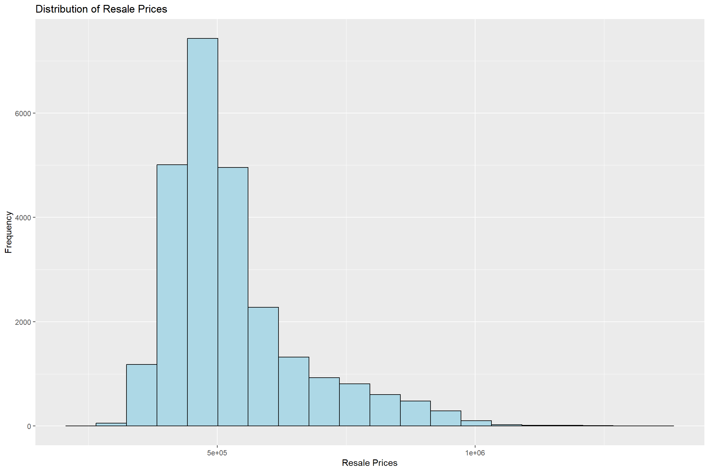
There appears to be a right-skewed distribution. This means that the majority of the housing prices are transacted on the lower end with some extremes.
Histogram Plotting of the Structural Factors
Extract the column names to plot
s_factors <- c("AREA_SQ", "LEASE_M", "age_of_unit", "storey_order")Create a list to store histograms on structural factors
Create a vector of the size of our structural vectors (4 in this case)
Plot the histogram for each structural factor
Append the histogram to the created vector
s_factor_hist_list <- vector(mode = "list", length = length(s_factors))
for (i in 1:length(s_factors)) {
hist_plot <- ggplot(final_resale_output, aes_string(x = s_factors[[i]])) +
geom_histogram(color="black", fill = "light blue") +
labs(title = s_factors[[i]]) +
theme(plot.title = element_text(size = 10),
axis.title = element_blank())
s_factor_hist_list[[i]] <- hist_plot
}Plot the histograms
We’ll use the ggarrange() function to organize them into a 2x2 column row plot.
ggarrange(plotlist = s_factor_hist_list,
ncol = 2,
nrow = 2)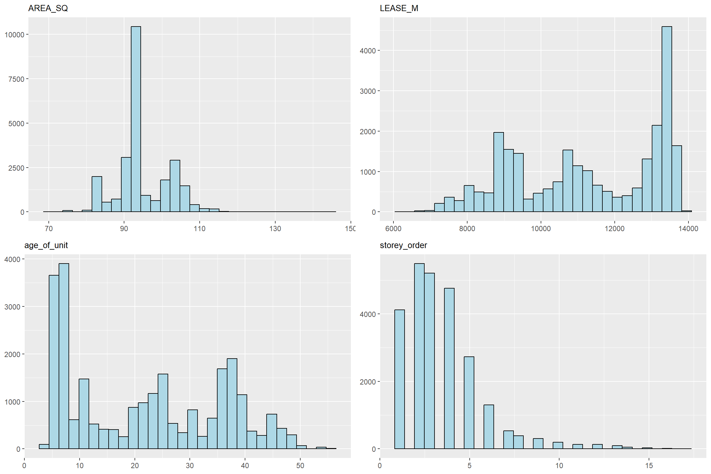
AREA_SQ:
It appears that most four-room flats roam around 90+ square feet. However, there are anomalies where it exceeds 110 square feet.
LEASE_M and Age of Unit
They appear to be inversely correlated. Where there is a large number of four-room flats that are not old and have a long lease life ahead.
Story Order:
There appear to be a familiar pattern where most of the four-room flats are built on lower floors. Though, this might be an effect where most HDBs are just built lower in general, with some anomalies of HDB flats which are built extremely high.
Locational Factors
l_factor <- c("PROX_CBD", "PROX_ELDERCARE", "PROX_HAWKER", "PROX_ISP", "PROX_MRT", "PROX_PARK", "PROX_TOP_PRI", "PROX_SHOPPING", "PROX_SUPERMARKET",
"NUM_KINDERGARTEN", "NUM_CHILDCARE", "NUM_BUS_STOPS", "NUM_PRI_SCHS", "NUM_TOURIST_SITES")l_factor_hist_list <- vector(mode = "list", length = length(l_factor))
for (i in 1:length(l_factor)) {
hist_plot <- ggplot(final_resale_output, aes_string(x = l_factor[[i]])) +
geom_histogram(color="midnight blue", fill = "light sky blue") +
labs(title = l_factor[[i]]) +
theme(plot.title = element_text(size = 10),
axis.title = element_blank())
l_factor_hist_list[[i]] <- hist_plot
}ggarrange(plotlist = l_factor_hist_list,
ncol= 4,
nrow = 4)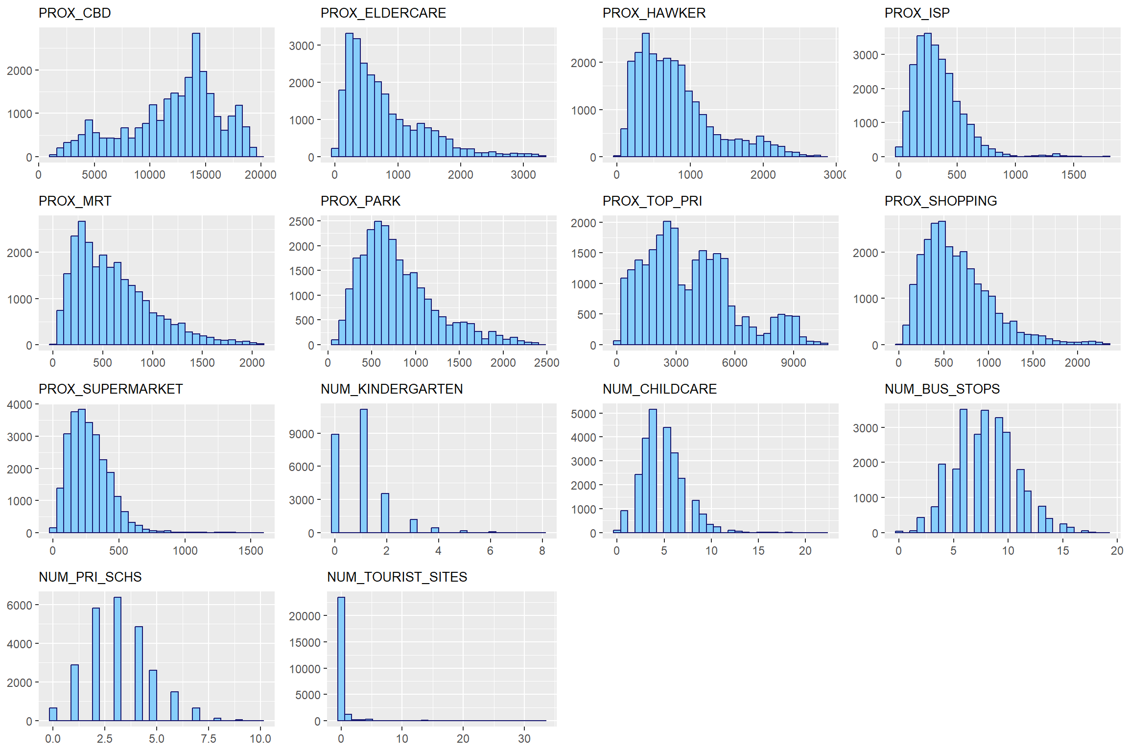
From observation, it appears that ELDERCARE are in the right-skewed in distribution. Which means some areas have a lot, while majority have almost none. Same goes for hawkers, ISP, MRT, PARK, SUPERMARKETS and shopping. This is a good thing, as this means most HDB are close to ISP, MRT, PARKS, SUPERMARKETS and shopping malls.
View the prices on the map:
tmap_mode("view")
tmap_options(check.and.fix = TRUE)
tm_shape(final_resale_output) +
tm_dots(col = "PRICE",
alpha = 0.6,
style="quantile") +
# sets minimum zoom level to 11, sets maximum zoom level to 14
tm_view(set.zoom.limits = c(11,14))